cheatsheet

Notebooks

• Colab notebook

Table of contents

1. Course syllabus and key points
2. Preview: Solving spam classification with optimization
3. Tentative course structure
4. Expectations and learning outcomes

Course syllabus and key points

Welcome to STAT 4830: Numerical optimization for data science and machine learning. This course teaches you how to formulate optimization problems, select and implement algorithms, and use frameworks like PyTorch to build and train models. Below are some highlights of the syllabus to get you oriented:

Prerequisites

• Basic calculus and linear algebra (Math 2400).
• Basic probability (Stat 4300).
• Familiarity with Python programming.
• You do not need a background in advanced optimization or machine learning research. We’ll cover the fundamentals together.

Schedule and format

• This is primarily a lecture-based course that will also include frequent group meetings with the professor.
• We will introduce theory (convexity, gradient-based methods, constraints, etc.) and then apply it in Python notebooks using PyTorch (and occasionally other libraries like CVXPY).

Deliverables

• A single final project that you begin drafting by Week 3 and refine throughout the semester.
• Several “checkpoints” (drafts, presentations) so you can get feedback and improve incrementally.
• The final submission will consist of a GitHub repository (code, report, slides) plus a polished demonstration (e.g., a Google Colab notebook).

Why PyTorch?

• We are focusing on PyTorch because deep learning’s success has been driven in part by modern auto-differentiation frameworks.
• These frameworks allow for rapid experimentation with new model architectures and optimization algorithms—something that older solver-based tools (like CVX or early MATLAB packages) did not fully accommodate.

Who is this course for?

• Targeted at junior/senior undergrads, but also valuable for PhD students wanting to incorporate numerical optimization into their research. Students who have met the prerequisites are welcome to join.
• If you already have a research project that involves model fitting or data analysis, this course may deepen your toolkit and sharpen your understanding of optimization.
• We will keep refining the course content based on your interests. If you have a particular topic, domain, or application you’d like to see, let me know.

A Brief History of Optimization

EVOLUTION OF OPTIMIZATION
========================

1950s                1960s-1990s              2000s                  TODAY
├─────────────────┐  ├────────────────┐  ┌────────────────┐  ┌─────────────────┐
│ LINEAR PROGRAM. │  │ CONVEX OPTIM.  │  │ SOLVER ERA     │  │ DEEP LEARNING   │
│ Dantzig's       │──│ Interior-point │--│ CVX & friends  │──│ PyTorch         │
│ Simplex Method  │  │ Large-scale    │  │ "Write it,     │  │ Custom losses   │
└─────────────────┘  └────────────────┘  │  solve it"     │  │ LLM boom        │
│                    │            └────────────────┘  └─────────────────┘
│                    │                   │                    │
▼                    ▼                   ▼                    ▼
APPLICATIONS:        APPLICATIONS:       APPLICATIONS:        APPLICATIONS:
• Logistics         • Control           • Signal Process    • Language Models
• Planning          • Networks          • Finance           • Image Gen
• Military          • Engineering       • Robotics          • RL & Control

It’s useful to appreciate how optimization evolved as an algorithmic discipline over the last seventy years:

• Mid-20th Century: Linear Programming emerged as a critical tool in operations research, fueled by George Dantzig’s simplex method. This was pivotal for industrial logistics, military planning, and resource allocation.
• 1960s–1990s: Convex optimization grew more important, driven by work on gradient-based methods, interior-point methods, and software that could solve large-scale linear and convex problems.
• 2000s: Tools like CVX (MATLAB-based) made formulating and solving standard convex problems more accessible to a broad audience—i.e., “specify your problem in a solver-friendly language, and let the solver handle it.”
• Modern Era: Deep learning frameworks (e.g., PyTorch, TensorFlow, Jax) have shifted the emphasis to a “build and iterate” approach. Instead of specifying problems in a polished convex form, we often “get our hands dirty” with nonconvex models, direct gradient-based methods, and custom loss functions. This iterative exploration is precisely what enabled the explosion of large language models (LLMs) and other powerful neural architectures.

In this course, we will appreciate both sides: solver-based approaches for classical, well-structured problems (via CVXPY) and more flexible, high-powered frameworks (via PyTorch) for data-driven, nonconvex tasks.

Preview: Solving spam classification with optimization

Let’s start with a classic problem: sorting important emails from spam.

The point of this preview is to show how a machine learning task turns into an optimization problem:

1. We define features: how an email becomes a vector $x$.
2. We define decision variables: weights $w$ that turn features into a prediction.
3. We define an objective: a loss function that scores the weights (cross-entropy).
4. We solve the optimization problem by minimizing the loss with gradient descent.

How computers read email

Consider two messages that land in your inbox:

email1 = """
Subject: URGENT! You've won $1,000,000!!!
Dear Friend! Act NOW to claim your PRIZE money!!!
Click here: www.totally-legit-prizes.com
"""

email2 = """
Subject: Team meeting tomorrow
Hi everyone, Just a reminder about our 2pm project sync.
Please review the attached agenda.
"""

Computers can’t directly understand text like we do. Instead, we convert each email into numbers called features. Think of features as measurements that help distinguish spam from real mail:

def extract_features(email, time_sent_hour):
keywords = {"urgent", "act", "now", "prize"}
tokens = set(email.lower().split())

features = {
'exclamation_count': email.count('!'),
'urgent_words': len(keywords & tokens),
'suspicious_links': sum('www' in token for token in email.split()),
'time_sent': time_sent_hour,   # Spam often sent at odd hours
'length': len(email),
}
return features

# Our spam email gets turned into numbers
spam_features = extract_features(email1, time_sent_hour=3)
print(spam_features)
# {'exclamation_count': 8,
#  'urgent_words': 3,
#  'suspicious_links': 1,
#  'time_sent': 3,
#  'length': 142}

From features to decisions

How do we decide if an email is spam? We assign a weight to each feature. Think of weights as measuring how suspicious each feature is:

import torch

weights = {
'exclamation_count': 0.5,    # More ! marks → more suspicious
'urgent_words': 0.8,         # "Urgent" language → very suspicious
'suspicious_links': 0.6,     # Unknown links → somewhat suspicious
'time_sent': 0.1,            # Time matters less
'length': -0.2               # Longer emails might be less suspicious
}

# PyTorch needs numbers in tensor form
features = torch.tensor([8.0, 3.0, 1.0, 3.0, 142.0])
w = torch.tensor(list(weights.values()), requires_grad=True)

The classification process

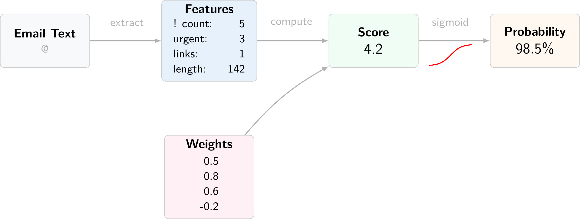
Features flow through a sequence of transformations:

1. Extract numeric features from raw text
2. Multiply each feature by its weight
3. Sum up the weighted features
4. Convert the sum to a probability using the sigmoid function

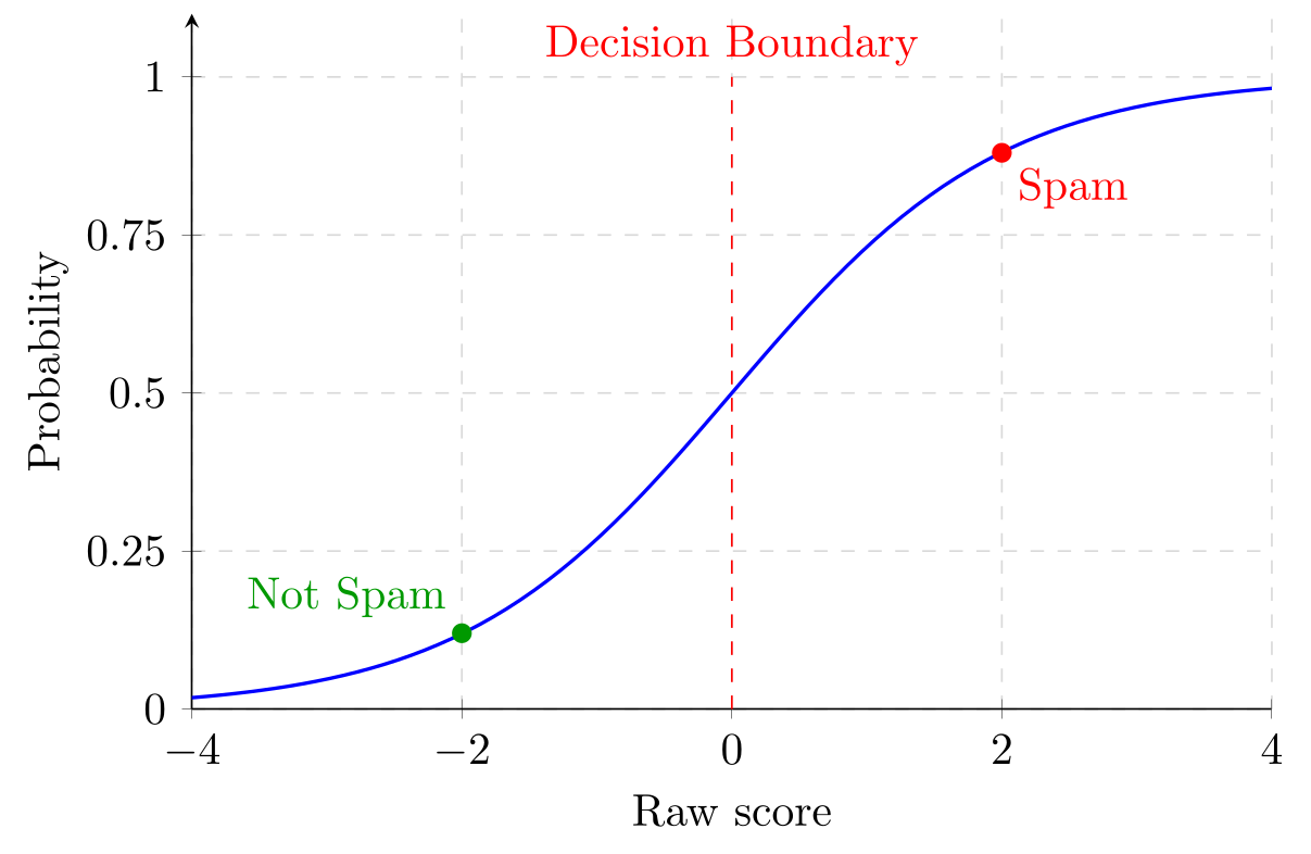
Making the decision: the sigmoid function

We combine features and weights to get a “spam score”. But how do we turn this score into a yes/no decision? We use a function called sigmoid that turns any number into a “probability” between 0 and 1:

def sigmoid(x):
return 1 / (1 + torch.exp(-x))

def spam_score(features, weights):
raw_score = torch.dot(features, weights)  # Combine features and weights
probability = sigmoid(raw_score)          # Convert to probability
return probability

The sigmoid function provides crucial properties:

• Very negative scores → probabilities near 0 (definitely not spam)
• Very positive scores → probabilities near 1 (definitely spam)
• Zero score → probability of 0.5 (maximum uncertainty)

The mathematical problem: finding optimal weights

Our spam filter needs to find weights that correctly classify emails. We can write this as an optimization problem:

[\min_{w}; L(w) := \frac{1}{n} \sum_{i=1}^{n \left[-y_i \log(\sigma(x_i}\top w)) - (1-y_i) \log(1-\sigma(x_i^\top w)) \right]]

Where:

• $w$ are the weights we’re trying to find (a vector with 5 entries)
• $x_i$ are the features of email $i$ (another vector with 5 entries)
• $x_i^\top w$ is the dot product of $x_i$ and $w$ (a scalar)
• $y_i$ is $1$ if email $i$ is spam, $0$ if not
• $\sigma$ is the sigmoid function
• $n$ is the number of training emails

This formula measures our mistakes (called “cross-entropy loss”).

Why cross-entropy is an appropriate loss function

The cross-entropy loss teaches our model to make confident, correct predictions while severely punishing mistakes. Let’s see how it works by examining the two curves in our plot, which show how we penalize predictions for spam and non-spam emails.

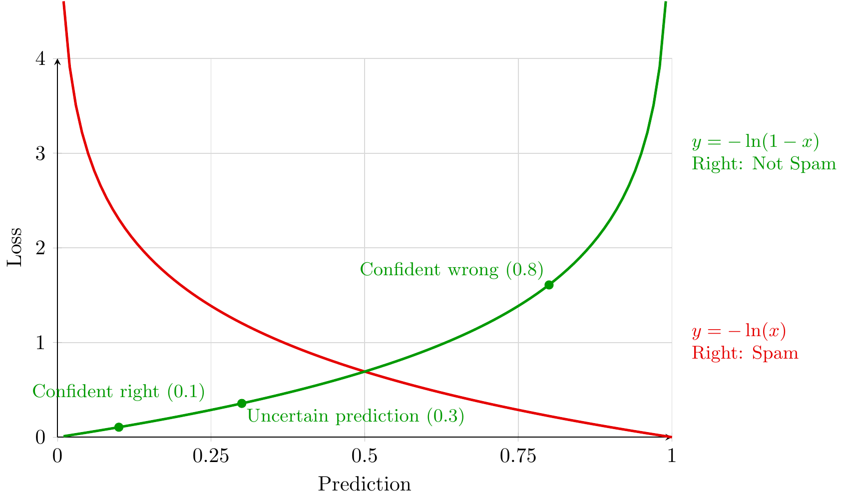
Consider a legitimate email (not spam, label = 0). Our model assigns it a probability of being spam:

uncertain_prediction = 0.3   # "Maybe spam (30% chance)?"
confident_wrong = 0.8       # "Probably spam (80% chance)"
confident_right = 0.1       # "Probably not spam (10% chance)"

The green curve (“Wrong: Not Spam”) shows how we penalize mistakes on legitimate emails:

• An uncertain wrong prediction (0.3) receives a moderate penalty
• A confident wrong prediction (0.8) triggers a severe penalty
• The penalty approaches infinity as the prediction approaches 1.0

The red curve (“Right: Spam”) works similarly but for actual spam emails. Together, the curves create a powerful learning dynamic:

Uncertainty gets corrected: The point “Uncertain & Wrong” shows a prediction hovering around 0.3 - not catastrophically wrong, but penalized enough to encourage learning. 1.

Confidence gets rewarded: The point “Confident & Right” shows a prediction around 0.1, receiving minimal penalty. This reinforces correct, confident predictions. 1.

Catastrophic mistakes get prevented: Both curves shoot upward at their edges, creating enormous penalties for high-confidence mistakes. This prevents the model from becoming overly confident in the wrong direction.

The two curves meet at 0.5 (our decision boundary), creating perfect symmetry between spam and non-spam mistakes. This balance means our model:

• Learns equally from both types of examples
• Develops appropriate uncertainty when evidence is weak
• Gains confidence only with strong supporting evidence

The mathematics behind this intuition uses the logarithm:

# For legitimate email (label = 0):
loss = -log(1 - prediction)   # Penalize high predictions

# For spam email (label = 1):
loss = -log(prediction)       # Penalize low predictions

Through training, these penalties push the average loss down by moving spam probabilities toward 1 on spam emails and toward 0 on non-spam emails:

# Before training (uncertain)
email1 = 0.48  # spam email, nearly random guess
email2 = 0.51  # non-spam email, nearly random guess

# After training (confident + correct)
email1 = 0.97  # spam email, high predicted probability of spam
email2 = 0.02  # non-spam email, low predicted probability of spam

How the optimization process works: gradients

At this point, we have an objective function $L(w)$ (the average cross-entropy loss on the training set). To find the minimum of the function, gradient methods follow the gradient of the function (or a modification thereof) towards the minimum. Why is this a reasonable strategy?

The gradient $\nabla L(w)$ is a vector of partial derivatives:

[\nabla L(w)=\left(\frac{\partial L}{\partial w_1},\ldots,\frac{\partial L}{\partial w_d}\right).]

It tells you how the loss changes if you nudge each weight coordinate.

The key idea behind gradient descent is the first-order Taylor approximation:

[L(w+\Delta)\approx L(w)+\langle \nabla L(w),\Delta\rangle .]

To make this approximation smaller, a natural choice is to move in a direction $\Delta$ that makes the inner product negative. The steepest instantaneous decrease (for a fixed step length) is achieved by taking $\Delta$ proportional to $-\nabla L(w)$.

That produces the update rule:

[w \leftarrow w - \eta \nabla L(w),]

equivalently

[w_j \leftarrow w_j - \eta \frac{\partial L}{\partial w_j}.]

Here $\eta > 0$ is called the learning rate or stepsize.

How much descent do we get from a step of gradient descent? If we take $\Delta = -\eta \nabla L(w)$ in the first-order approximation

[L(w-\eta \nabla L(w)) \approx L(w) - \eta \langle \nabla L(w),\nabla L(w)\rangle = L(w) - \eta |\nabla L(w)|^2.]

So, for small enough $\eta>0$, stepping in the negative gradient direction decreases the loss to first order.

A dramatically oversimplified picture of gradient descent is that we are walking downhill on a surface and the gradient always points towards the current steepest direction downwards. In reality there are many obstacles to reaching the minimum, including local minima, saddle points, and even ravines

Gradient descent path (cartoon).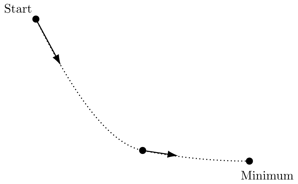

Saddle point example.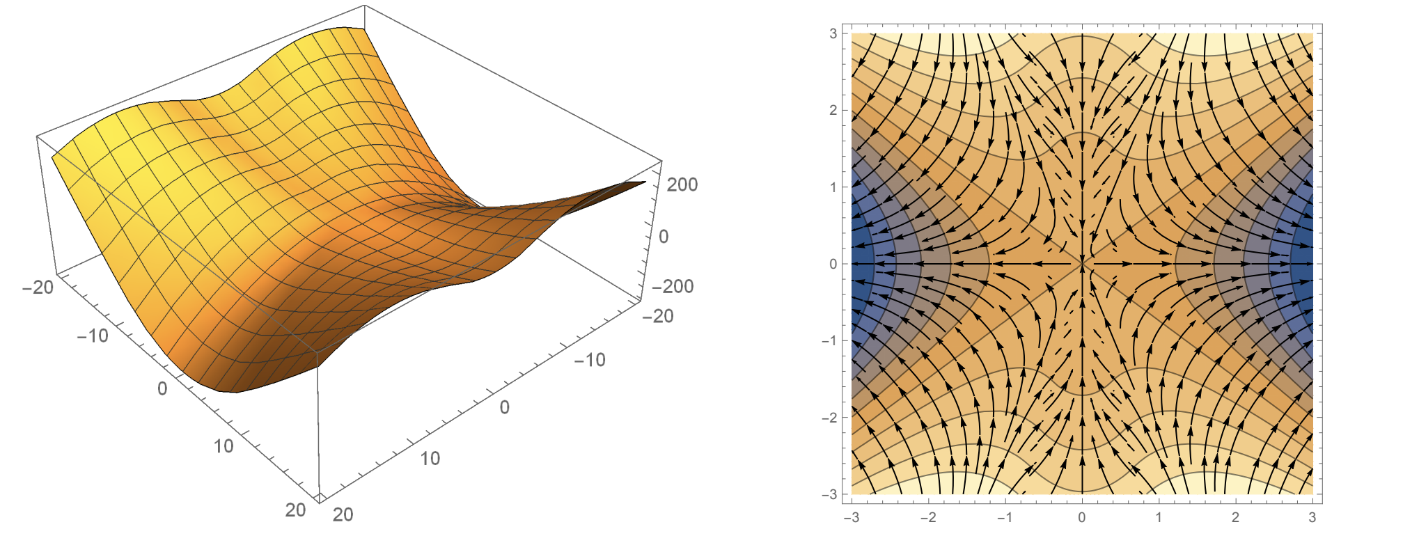

Ravine example.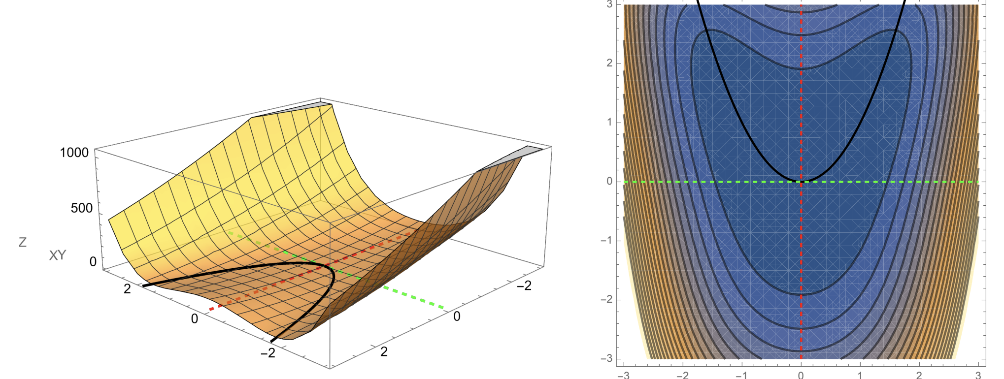

Finding the weights with PyTorch

In PyTorch, loss.backward() computes $\nabla L(w)$ for you and stores it in weights.grad. The update line weights -= learning_rate * weights.grad is exactly the gradient descent update $w \leftarrow w - \eta \nabla L(w)$.

# Start with random weights
weights = torch.randn(5, requires_grad=True)
learning_rate = 0.01

for _ in range(1000):
# 1. Make predictions and calculate mistakes
predictions = spam_score(features, weights)
loss = cross_entropy_loss(predictions, true_labels)

# 2. Calculate gradient (steepest direction)
loss.backward()

# 3. Take a step downhill
with torch.no_grad():
weights -= learning_rate * weights.grad
weights.grad.zero_()

Two details matter here:

• loss.backward() computes all partial derivatives and puts them into weights.grad.
• We reset gradients with weights.grad.zero_() because PyTorch accumulates gradients by default.

The loop above runs a fixed number of steps. Other stopping rules are common (stop when the loss plateaus, stop after a fixed time budget, stop after a target accuracy).

Numerical results

When you checkout the notebook for this lecture, this is what you’ll see as you run the training loop: 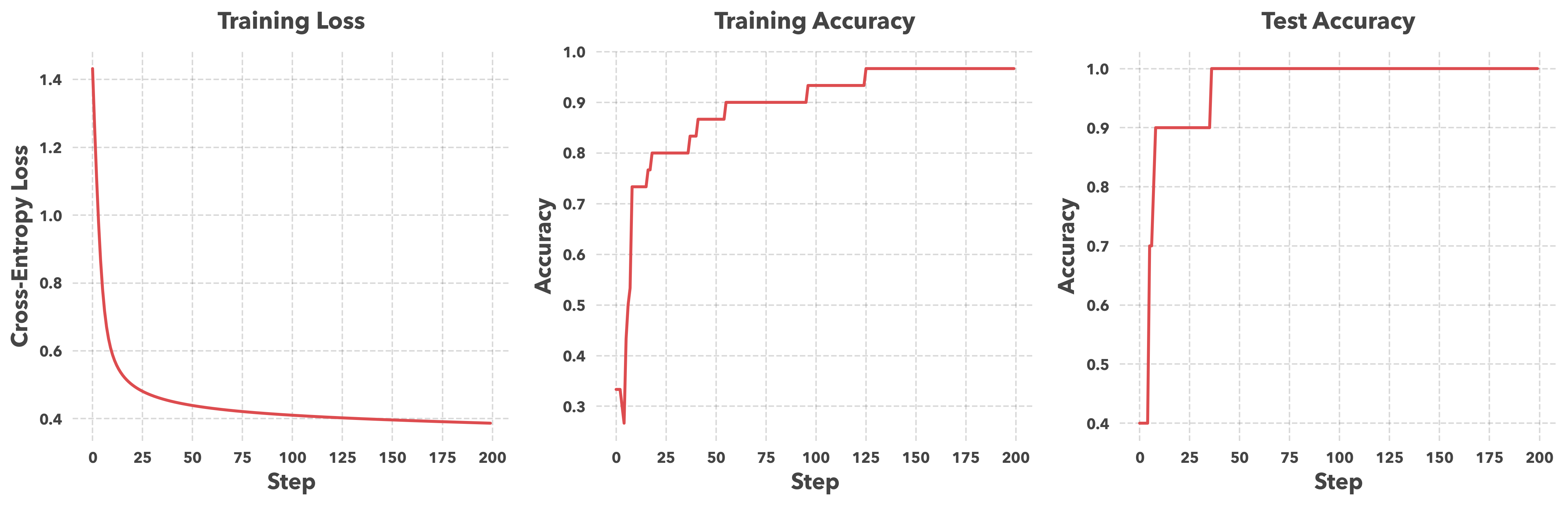The first plot shows the value of the cross-entropy loss as we train the model. This and the “training accuracy” (shown in the second plot) are diagnostics: they show whether the optimization loop is reducing the objective on the training set.

The third plot is the test accuracy, computed on emails that were not used to train the model. A key goal in machine learning is for our our performance on the training set to generalize to the test set. A large gap between training and test accuracy would suggest overfitting. In this run, the training and test curves are close and stabilize, so these plots do not show an obvious generalization gap for this dataset.

The what, how, and why of PyTorch

Once you write down a loss $L(w)$, gradient descent needs $\nabla L(w)$. For realistic models, computing gradients by hand is tedious and error-prone.

PyTorch computes gradients automatically. If you build a scalar-valued loss using PyTorch operations, PyTorch records the operations used to compute that loss. When you call backward(), it applies the chain rule through that recorded computation and produces derivatives with respect to any variables that have requires_grad=True.

Here is a one-dimensional example where you can see the chain rule explicitly. Fix a number $y$ and define

[f(x) = (x^2 - y)^2.]

Write this as a composition: $h(x)=x^2$ and $g(z)=(z-y)^2$, so $f=g\circ h$. The chain rule gives

[f’(x) = g’(h(x))h’(x) = 2(x^2-y)\cdot 2x = 4x(x^2-y).]

PyTorch computes the same derivative automatically because it tracks the operations used to build the function $f$:

import torch

y = 3.0
x = torch.tensor(2.0, requires_grad=True)

f = (x**2 - y)**2
f.backward()

print("f(x) =", f.item())
print("df/dx =", x.grad.item())  # 4*x*(x**2 - y)

The practical payoff is that we can change the model or the loss and keep the same optimization loop. We will use that constantly in this course.

What you’ll learn in this course

This spam filter example is intentionally simple, but it has the same structure as most machine learning problems:

• represent data as vectors (features),
• choose parameters $w$ that produce predictions,
• define an objective $L(w)$ that measures performance,
• compute $\nabla L(w)$ and update $w$ with a gradient-based method.

Throughout this course and especially in your projects, you will execute thse same four steps. While they seem straightforward in this example, they require extensive tuning, and have a surprising amount of detail.

Tentative course structure

This is my second time teaching this course. You may find the first version of this course here. I’m significantly revamping this course based on student feedback to make the lectures quickly relevant to your final projects. Below is the current structure that I’ve settled on, but the content may shift.

We start in one dimension. We will define the decision variable, the loss function, and what we mean by an approximate minimizer. We will derive why gradients are the right primitive, write down gradient descent and stochastic gradient descent explicitly, and implement them twice: first by hand in NumPy, then using automatic differentiation in PyTorch. We will discuss how PyTorch computes gradients via autodifferentiaion. We will also discuss basic hyperparameter tuning strategies. Finally, we will touch on constraints early, because many practical problems come with them.

Next we move to higher dimensions and build the linear algebra interface we need in PyTorch: tensors, norms, inner products, and matrix products. We will talk about efficiency as it shows up in code, including broadcasting and memory layout. We will also use SVD as a first tool for looking at structure in data.

With that tooling, we will build a menu of problems in signal processing, machine learning, and reinforcement learning and focus on how to formulate them cleanly in code. We will look at classical ML problems (linear and logistic regression, SVMs), modern deep learning problems (neural networks, transformers, diffusion models), and a few inverse problems (compressed sensing, phase retrieval, low-rank recovery). We wil also provide a quick introduction to RL problems as they’re currently being used in large language models. Finally, we introduce classical optimization templates (LPs, QPs, SDPs) and describe how one can solve them with existing solver-based workflows (CVXPY and solvers such as Clarabel).

Once you can formulate problems, we will treat algorithms as objects with an API: what update they implement, what hyperparameters they expose, and what regimes they tend to work in. We will cover gradient descent, stochastic gradient descent, Adam and AdamW, and a handful of other methods that show up in current practice (SignGD, Muon, Shampoo). We will also discuss modifiers like weight decay, EMA, momentum, batch size, and constraints.

Then we will shift to benchmarking and tuning methods. We will learn how to run comparisons that answer a question (time-to-result, final accuracy, stability) rather than comparisons that just produce a nice plot. Some of this material will draw from the previous course benchmarking notes (e.g., section 10 notes and section 11 notes.

Next, we will take a brief look at ML systems. We will describe how to think about GPUs, the core accelerator of modern ML research. We will also talk about how one trains large-scale models over multiple GPUs.

Finally, we will discuss what theory can tell us. We will highlight the differences between convexity and nonconvexity, how conditioning impacts algorithmic speed, and, provide complexity estimates for GD and SGD. We will also introduce a few simple, but predictive models for deep learning: random features, noisy quadratic models, mean estimation. Finally we will briefly discuss scaling laws and MuP as heuristics for scaling large models.

Expectations and learning outcomes

By the end of the course, you should be able to do the following.

Formulate optimization problems. Identify decision variables, objectives, and constraints for a given problem, and write them down clearly in both math and code. 1.

Implement and debug gradient-based training loops in PyTorch. Build a model, compute a loss, call backward(), update parameters, and debug common failure modes. 1.

Choose reasonable algorithms and hyperparameters. Know when to start with GD/SGD/Adam. Understand what learning rate, batch size, momentum, and weight decay are doing. Recognize symptoms of bad tuning (divergence, noise floor, slow progress). 1.

Benchmark methods in a way that is not misleading. Run fair comparisons and report results that answer a question (time-to-result, final accuracy, stability). 1.

Have basic systems awareness. Understand when compute, memory, or data loading is the bottleneck. Have a working vocabulary for GPUs and lightweight distributed training, even if you do not implement full-scale systems. 1.

Produce a portfolio-quality project. Build a clean repo with a clear objective, a working implementation, and a short write-up that explains what you did and what worked.