In “black-widow” systems, a millisecond pulsar is orbited closely (Porb < 1 day) by a low-mass (<0.1 M⊙), often-degenerate companion. They are so named because in a prior low-mass X-ray binary phase, the pulsar was spun up by accreting mass from the companion, while at present the companions are being evaporated by the pulsar. There are ∼50 known black-widow systems (K. I. I. Koljonen & M. Linares 2025), several of which have estimated companion masses below 10 MJ. Of the handful with short (≲ few days) orbital periods, only one has a minimum density similar to that of gas giants orbiting main-sequence stars: PSR J2322–2650b (R. Spiewak et al. 2017; M. Shamohammadi et al. 2024), with a minimum mass of…
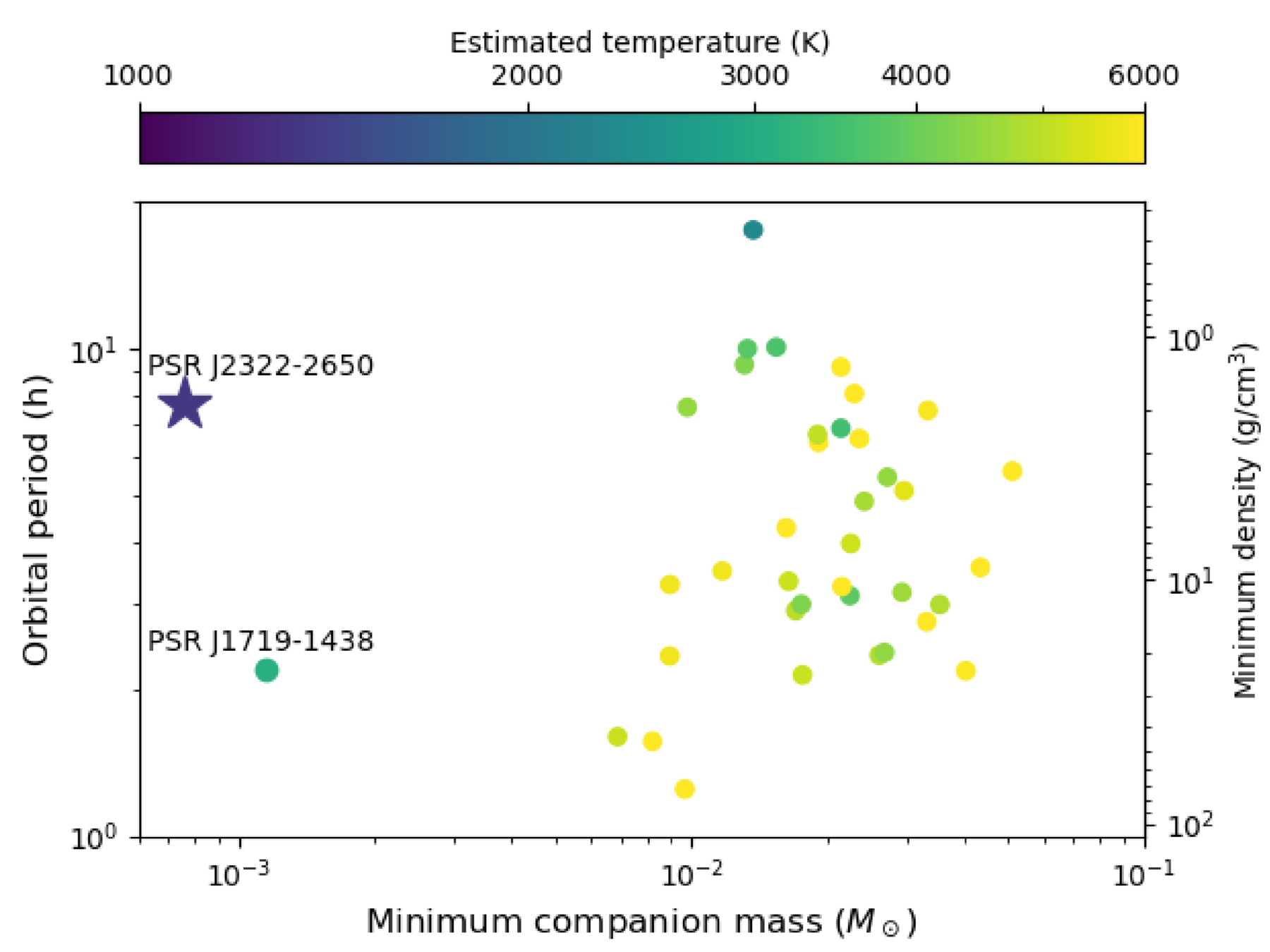
In “black-widow” systems, a millisecond pulsar is orbited closely (Porb < 1 day) by a low-mass (<0.1 M⊙), often-degenerate companion. They are so named because in a prior low-mass X-ray binary phase, the pulsar was spun up by accreting mass from the companion, while at present the companions are being evaporated by the pulsar. There are ∼50 known black-widow systems (K. I. I. Koljonen & M. Linares 2025), several of which have estimated companion masses below 10 MJ. Of the handful with short (≲ few days) orbital periods, only one has a minimum density similar to that of gas giants orbiting main-sequence stars: PSR J2322–2650b (R. Spiewak et al. 2017; M. Shamohammadi et al. 2024), with a minimum mass of 0.8 MJ and a minimum density of 1.8 g cm−3. The pulsar’s unusually low spindown luminosity of 2 × 1032 erg s−1—arising from its unusually low magnetic field—would give the companion an equilibrium temperature of 1300 K if isotropically radiated and fully converted to heat. However, the gamma rays that dominate a millisecond pulsar’s energy output and are responsible for heating the companion are typically beamed toward the equator (e.g., A. Philippov et al. 2020), making an accurate prediction of the companion temperature difficult.
The atmospheres of a few of PSR J2322–2650b’s denser and more massive black-widow cousins have been studied from the ground (e.g., P. Draghis et al. 2019; D. Kandel & R. W. Romani 2020; V. S. Dhillon et al. 2022). D. Kandel & R. W. Romani (2023) summarize 10 sets of previously published photometric phase curves of black-widow companions, with masses ranging from 12 to 67 MJ and densities ranging from 20 to 40 g cm−3. All are extremely hot—nine have nightside temperatures above 2200 K, while J1311–3430 has no detectable nightside emission, but its dayside is >10,000 K. These studies have measured the atmospheric circulation, Roche-lobe fill factors, and inclinations of these extreme objects. They have even provided tentative estimates of pulsar masses and put constraints on the neutron star equation of state. Spectra have been taken of several black-widow companions (e.g., M. H. van Kerkwijk et al. 2011; R. W. Romani et al. 2015, 2016, 2022; M. R. Kennedy et al. 2022; J. A. Simpson et al. 2025) and are generally stellar, indicating roughly solar composition. However, J1311–3430 and J1653–0158 both have 10–15MJ companions with H-free surface spectra; these represent a black-widow subclass, the “Tidarrens,” which are likely descendants of ultracompact low-mass X-ray binaries with evolved companions (R. W. Romani et al. 2015). Y. Guo et al. (2022) showed with MESA simulations that these ultralight companions—including PSR J1719–1438, J2322–2650, and J1311–3430—could have formed by the Roche-lobe overflow and photoevaporation of helium stars.
PSR J2322–2650b is different from other ultralight pulsar companions, being the only pulsar companion with a mass, a density, and a temperature similar to those of hot Jupiters (Figure 1). The atmosphere of such an object has never been observed. It is, however, very easily observable with JWST: at infrared wavelengths, the pulsar is undetectable, giving us the unprecedented opportunity to obtain exquisite spectra of an externally irradiated planetary mass object. In this Letter, we present JWST spectra of this exotic gamma-ray-heated “exoplanet,” unveiling a bizarre atmosphere that raises more questions than it answers.
Figure 1. PSR J2322–2650 compared to the black widows from SpiderCat (K. I. I. Koljonen & M. Linares 2025) and to PSR J1719–1438 (M. Bailes et al. 2011), showing it is in a distinct area of parameter space. PSR J1719–1438, though similar in mass, has a much higher mean density of 21 g cm−3; its bulk composition is likely very different. The temperatures of all companions were very roughly estimated by assuming the spindown luminosity is isotropically radiated and all of the energy hitting the companion is converted to heat. The minimum density was derived from the orbital period via  , combining Paczyński’s approximation for the Roche lobe (R**L = 0.463q1/3a; B. Paczyński 1971) with Kepler’s third law.
Download figure:
Standard image High-resolution image
On 2024 November 8, we used NIRSpec/PRISM on JWST to observe PSR J2322–2650b’s 0.6–5.3 μm spectroscopic phase curve. These observations started shortly before inferior conjunction (the “nightside”) and continued until shortly after the following inferior conjunction, covering the whole 7.8 hr orbit. Two days later, we used NIRSpec/G235H (1.7–3.1 μm) to take a 2 hr long higher-resolution spectral sequence bracketing superior conjunction (the “dayside”). This data set spans an orbital phase range of 0.25, allowing us to measure the radial velocity of the planet as a function of time. Both the PRISM and G235H observations are taken with the 0 2 fixed slit. All the JWST data used in this Letter can be found at MAST: doi:10.17909/shv0-yq03. We develop a custom pipeline to reduce the data, significantly reducing the scatter compared to JWST standard pipeline processing (see Appendix B).
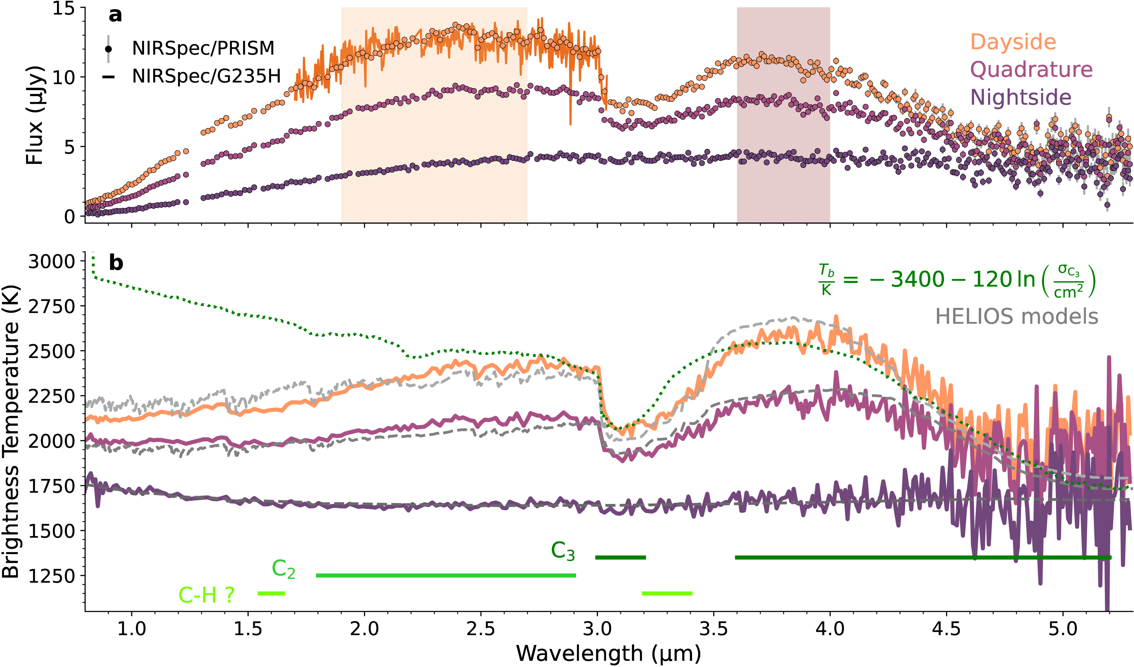
We show in Figure 2 the average PRISM spectrum on the dayside, quadrature, and nightside (defined as phases 0.5 ± 0.085, 0.25 ± 0.05 or 0.75 ± 0.05, and 0.00 ± 0.05 or 1.00 ± 0.05, respectively). The spectra are shown both in μJy and in brightness temperature, calculated with a fiducial radius of 1.1RJ and an updated radio pulsar timing parallax distance of 630 pc (see Appendix A). While the nightside spectrum is featureless and consistent with a near-isothermal temperature profile or a thick gray dust/cloud deck, the dayside spectrum has clear absorption features. We can identify the molecules giving rise to these features by comparing the brightness temperature spectrum against  , where σ(λ) is the absorption cross section of a candidate molecule. After a complete search of the DACE17 molecular database and an extensive search of the ExoMol (J. Tennyson & S. N. Yurchenko 2018) molecular database, we conclude that C3 and C2 are firmly detected. As shown in Figure 2, the cross section of 12C3 (A. E. Lynas-Gray et al. 2024) rises suddenly redward of 3.014 μm, matching the sudden flux drop seen in the data. (The isotopologues 12C13C12C and 12C12C13C have opacity cliffs at slightly different wavelengths and are inconsistent with the data, but their line lists are less reliable because they are not matched to experiments.) C3 also has an opacity minimum at 3.9 μm, matching the maximum in the emission spectrum, and an opacity maximum at 5.1 μm, matching the emission plateau. The sawtooth pattern at 2.45–2.85 μm matches the series of band heads in the opacity of C2 (S. N. Yurchenko et al. 2018).
Figure 2. The observed emission flux and brightness temperature of PSR J2322–2650b. (a) Observed PRISM spectrum of the dayside, the average of the two quadratures, and the nightside at native resolution. The time-averaged G235H spectrum is also plotted, binned in wavelength by a factor of 16. The two shaded wavelength regions are those of the light curves in Figure 5. (b) PRISM spectra expressed in brightness temperatures by assuming R/D = (1.1 RJ) / (630 pc). We plot HELIOS radiative-convective equilibrium forward models in gray. A linear function of the log of C3’s absorption cross sections is plotted in green, showing that C3 absorption explains the sudden dip at 3.014 um, the recovery at 4 um, and the slow decline toward the red edge.
Download figure:
Standard image High-resolution image 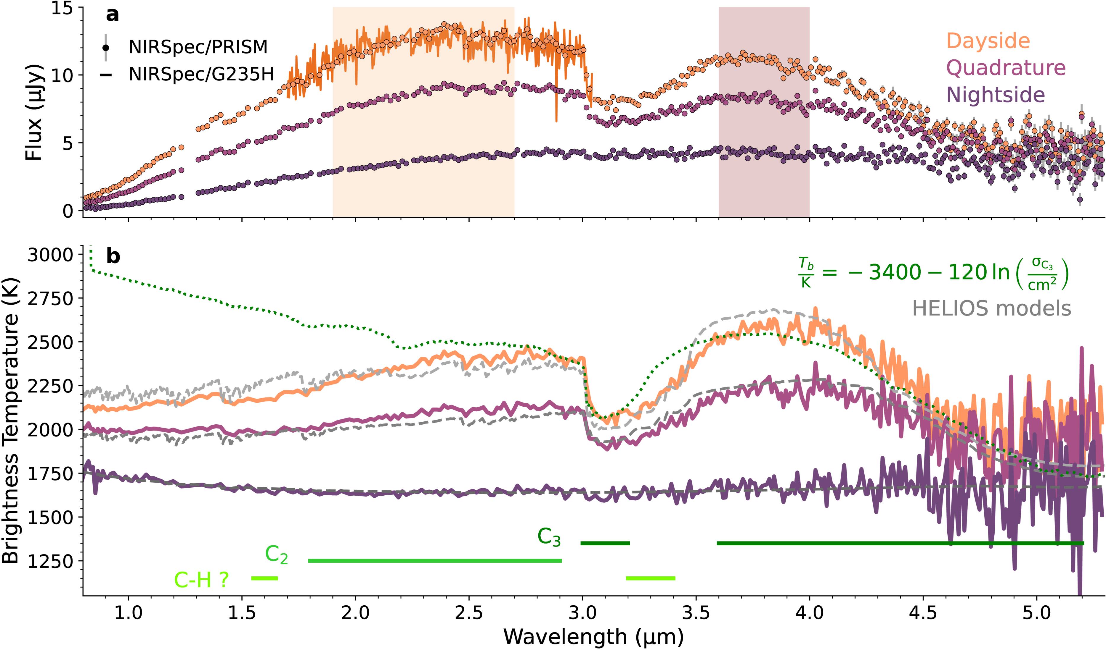
C3 and C2 are necessary but not sufficient to explain the PRISM spectrum. First, the absorption feature at 3.0–3.6 μm is wider than the C3 opacity peak, requiring another source of opacity around 3.4 μm. Similarly, while a C2 opacity peak around 1.4 μm could explain the sudden drop in flux at that wavelength, the absorption feature extends much redder than the opacity peak, suggesting that there is missing opacity around 1.6 μm. We confirm that isotopologues of C3 and C2 cannot explain the missing opacity at either wavelength and tentatively identify both absorption features as arising from the C–H bond. The fundamental stretching mode of this bond is at 3.4 μm, resulting in the ubiquitous presence of absorption at this wavelength among organic molecules (see Table 1.2 of M. Tammer 2004). The first overtone of the 3.4 μm stretch mode is at half the wavelength, or 1.7 μm. Due to the similarity of absorption features across large classes of organic molecules, the exact molecule(s) giving rise to the C–H absorption is difficult to determine. We consider the identification of the features as C–H absorption to be tentative, because we detect no absorption feature around 2.3 μm, whereas such a feature is common in hydrocarbons.
While the sawtooth feature in the PRISM spectrum strongly hints at the existence of C2, the higher-resolution G235H spectra conclusively demonstrate its existence. Using techniques from high-resolution cross-correlation spectroscopy (I. Snellen 2025), we cross-correlate the smoothed logarithm of C2 opacities with each of the 151 integrations in the grating observation (see Appendix F). Plotting the cross-correlation function (CCF) with respect to time and blueshift reveals the radial velocity track of the planet. Given an assumed projected orbital velocity K**p and barycenter velocity vsys, we can shift the CCFs into the planetary frame and sum them along the time axis to obtain a C2 detection significance. Maximizing this significance over the K**p–vsys plane, as shown in the left panel of Figure 3, yields a 21σ detection of C2 at a barycentric velocity close to 0 and a projected orbital velocity K**p ∼ 200 km s−1.
Figure 3. C2 detection significance and radial velocities obtained from the JWST NIRSpec/G235H data. (a) The detection significance from the cross-correlation of C2 in the G235H data, as a function of projected orbital velocity and barycentric radial velocity. C2 is detected at 21σ at Vsys ≈ 0 and Kcomp = 190 km s−1. (b) In black, the companion radial velocity measured from each integration of the G235H observations using a data-derived template; in yellow, a sinusoidal fit to the data. The vertical offset is arbitrary. In the colored bars, we show the phases we define to be the nightside, quadrature, and dayside, for the purposes of calculating the average spectra in Figure 2.
Download figure:
Standard image High-resolution image 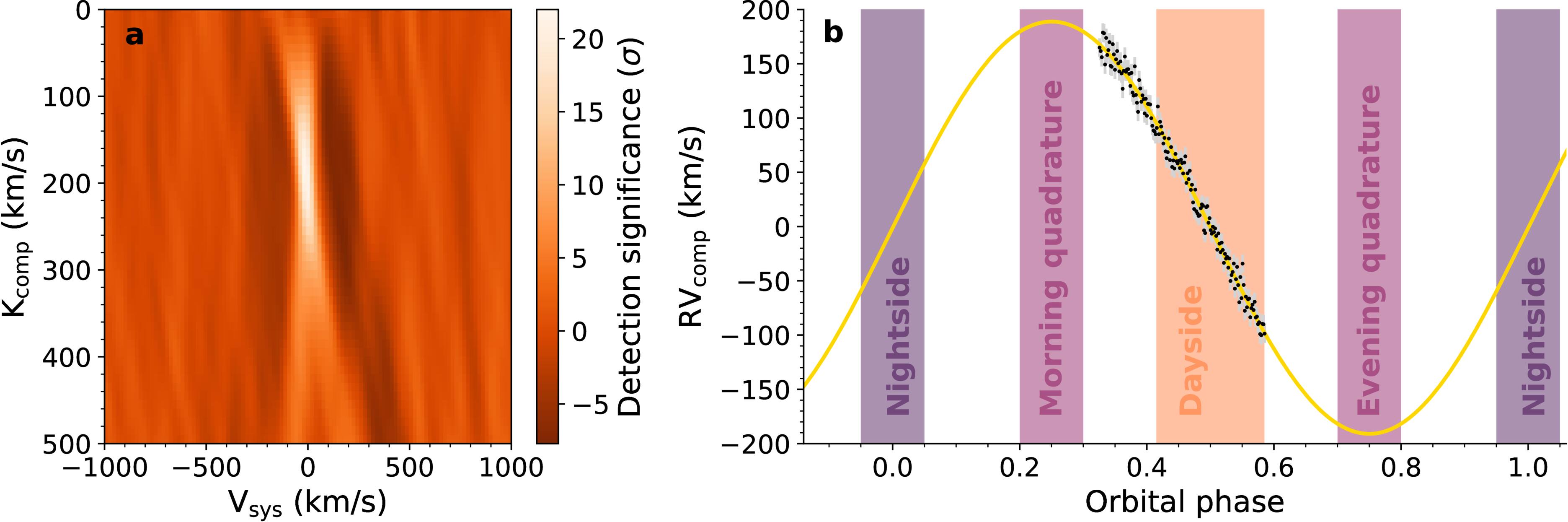
In exoplanetary atmospheres, carbon-bearing molecules such as CO, CH4, and CO2 are commonly detected, but molecular carbon has never been seen. To quantify how depleted the atmosphere is in noncarbon elements, we obtain robust model-independent constraints on molecular abundance ratios by constructing a simulated G235H spectrum from only the cross sections of C2 and a non-C2 molecule, adjusting the line contrast until C2 is detected at the same significance as in the real data, and computing the detection significance of the other molecule. As detailed in Appendix F, we perform this procedure with C2/CO using the 2.30–2.47 μm range, where both molecules have substantial opacity, and we find a 3σ lower limit on C2/CO of 0.17. We repeat the procedure with CN, which has higher opacity than CO over a larger wavelength range, finding C2/CN > 32 at 3.2σ. We additionally search for a wide variety of other molecules in the grating data via cross-correlation—including CS, CH, NS, OCS, H2O, and CH4—but find no >3σ detections.
Our inferred abundances suggest an atmosphere rich in carbon and relatively depleted in oxygen and nitrogen. Hydrogen is also heavily depleted, as otherwise the ample carbon atoms would bond with H to form hydrocarbons, resulting in minuscule abundances of molecular carbon, as has been predicted for hot-Jupiter exoplanets with high C/O ratios (N. Madhusudhan 2012). Some C–H features are still possible, however, as trace amounts of hydrogen can be produced via spallation by the pulsar wind (B. M. S. Hansen 1996). On the other hand, this object is unlikely to be dominated by carbon in bulk, due to its equation of state. To test this, we calculate the mass–radius relationship of a pure carbon object using an interior structure model (M. C. Nixon & N. Madhusudhan 2021; M. C. Nixon et al. 2024) with the equation of state of G. I. Kerley & L. Chhabildas (2001) (see Appendix C) and find that, at zero temperature, the radius of a 1.5–2.5 MJ object (0.39 RJ) is much smaller than the near-Roche-lobe-filling radius our PRISM phase curve requires (see Section 5). A central temperature of 500,000 K would be needed to inflate a carbon object to a Jupiter radius, but this is unrealistically hot, given (as we will later argue) its likely past as a white dwarf with efficient conductive heat transport. If, however, we assume an object that is mostly helium, with 1% C, then the radius increases to 0.92 RJ for a 1.5 MJ object with a photosphere temperature of 1500 K, using the helium equation of state from G. Chabrier & F. Debras (2021) and an additive volume law. We thus conclude that the planet’s bulk composition is likely helium-dominated.
3.1. Equilibrium Chemistry
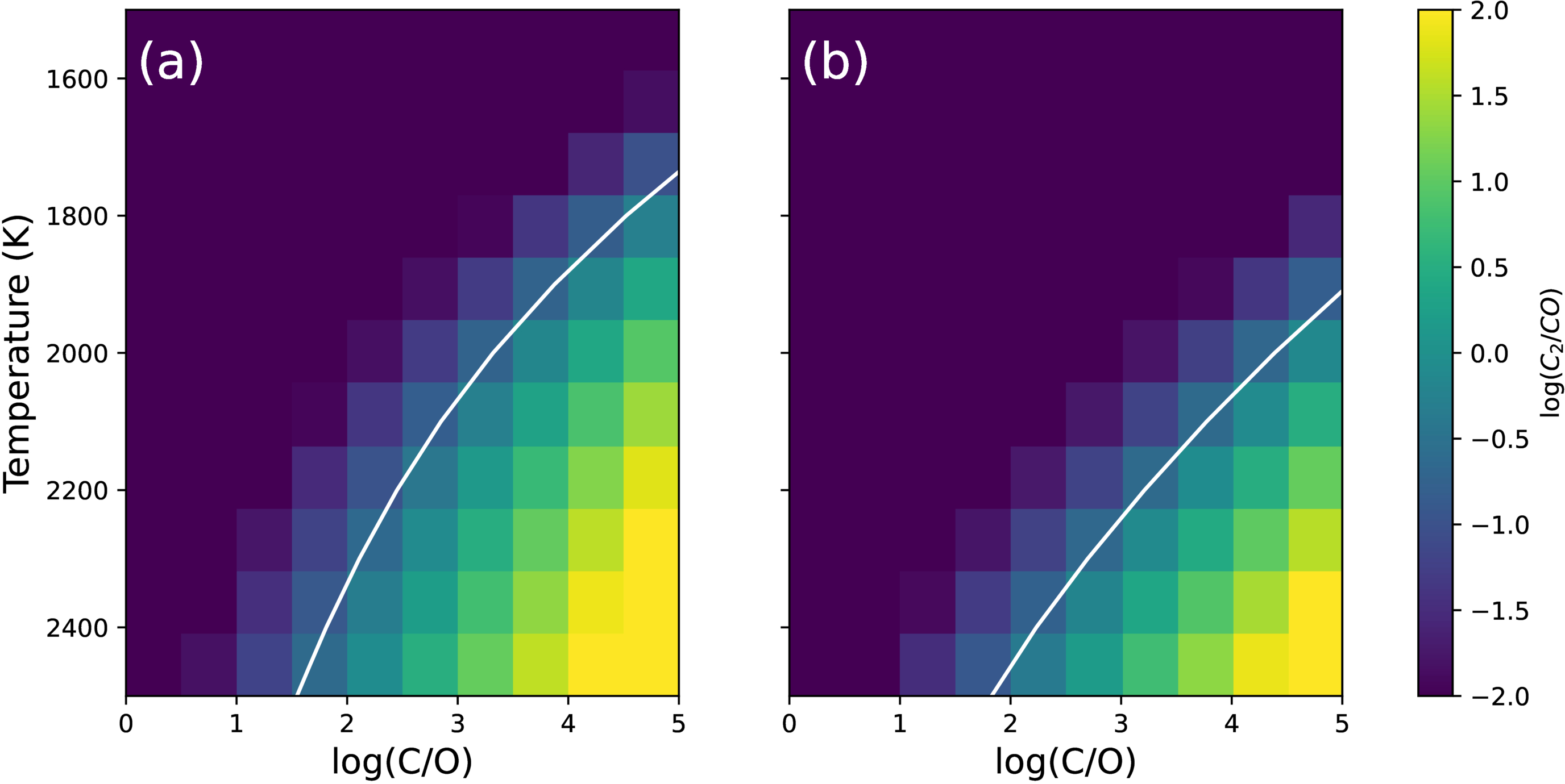
We can test whether a helium-dominated atmosphere enriched in carbon can reproduce our observations by performing equilibrium chemistry calculations with FastChem (J. W. Stock et al. 2018, 2022). Figure 4 plots the ratio of C2/CO as a function of temperature and atomic C/O, either assuming C/He = 0.01 and no other elements or assuming H/He = 0.01 as well as solar N/He, P/He, and S/He. In either case, CO is highly favored over C2 until C/O ≫ 1 and far more favored at low temperatures. Even at 2300 K, the hottest point in our ICARUS model (see below), our constraint of C2/CO > 0.17 requires C/O > 100. At the average dayside brightness temperature of 2000 K, C2/CO > 0.17 would require C/O > 2000 (the pure-He-and-C scenario) or C/O > 20,000 (the many-elements scenario). We generate multidimensional abundance grids to explore a wide range of metallicities, C/O and C/N ratios, temperatures, and pressures, finding that our observational constraints on C2/CO and C2/CN imply C/O > 100 and C/N > 10,000 over a wide range of conditions (see Appendix H).
Figure 4. The relative abundance of C2 to CO in chemical equilibrium. (a) Abundance ratios for C/He = 10−2 and P = 10 mbar, for an atmosphere with no other elements. (b) Ratios in an atmosphere with H/He = 0.01 as well as solar values of N/He, P/He, and S/He. The solid white curves represent the 3σ constraint from our cross-correlation test (C2/CO > 0.17).
Download figure:
Standard image High-resolution image 
In our high-C/O calculations with only C, O, and He, C3 is the most abundant molecule, consistent with our observations; at C/O ∼ 1, CO is the most abundant molecule and C3 has negligible (parts per billion or less) abundances. In our calculations including hydrogen and other elements, C3H and C2H are comparably abundant to C3 and C2 over a wide range of temperatures and C/O ratios. The C–H bonds on these molecules may explain the opacity we see at 3.4 and 1.6 μm, but since there are no published line lists for these molecules, we are unable to include them in our modeling. Colder carbon-rich compositions (T < 1000 K, C/O ≫ 1) are predicted to have abundant quantities of larger carbon molecules, such as C4 and C5, which also have no published line lists. To compare these results to data, we generate forward models using HELIOS (M. Malik et al. 2017, 2019; see Appendix D), assuming 1D radiative-convective equilibrium in a bottom-heated helium-dominated atmosphere with an extended graphite dust/cloud layer and ∼part per thousand abundances of C3, C2, and C2H4 (a stand-in for a generic molecule with C–H bonds). These are shown in Figure 2, which demonstrates that this simple prescription reproduces the main spectral features at all phases, with the featureless nightside explained by invoking more dust absorption.
Refining the value of the projected orbital velocity K**p allows us to pin down the inclination of the companion orbit and the masses of the companion and pulsar, as well as assess the validity of our fiducial companion radius. We use the G235H spectra to monitor the radial velocity variations (D. K. Sing et al. 2024). We generate a template spectrum by shifting every spectrum into the planetary frame using our preliminary K**p value (∼200 km s−1) and taking the timewise average. We then fit this template to each individual spectrum to find the radial velocity shift as a function of time, as shown in Figure 3 (right). Finally, we fit the sinusoid  to the velocities. We obtain K**p = 190 ± 2 km s−1. This value represents the center-of-light orbital velocity KCoL, which is lower than the planet’s center-of-mass orbital velocity KCoM, because the bright, irradiated side of the planet is closer to the pulsar. The ratio Kcor = KCoM/KCoL depends on the heating pattern, temperature dependence of the lines dominating the radial velocity, Roche-lobe fill factor, and inclination. For our system with its mass ratio q ≈ 1000, the maximum possible value of Kcor is 1/(1 − (3q)−1/3) = 1.07, which reduces to 1.04 for a more realistic
  temperature distribution (M. H. van Kerkwijk et al. 2011).
For a binary system in a circular orbit where the primary is much more massive than the secondary,  . Assuming the pulsar mass M**p can range from the canonical 1.4M⊙ to an unusually massive 2.4M⊙ (see Figure 7 of J. M. Lattimer 2012), we infer an inclination range of 34
 7–28
7–28 4 (for Kcor = 1.04). This low i, combined with the fact that pulsar gamma rays are beamed toward the spin equator, explains a number of system features: the lack of a Fermi gamma-ray detection (S. Abdollahi et al. 2022), the high companion temperature compared to the pulsar spindown power, and the lack of radio eclipses from a companion outflow. This range of inclinations implies a planet mass of 1.4–2.4MJ, a Roche-lobe radius
  of 0.99–1.18RJ, and density of 1.8 g cm−3. All plausible pulsar masses therefore imply a roughly Jupiter-sized and Jupiter-mass companion on a ∼30∘ inclination orbit.
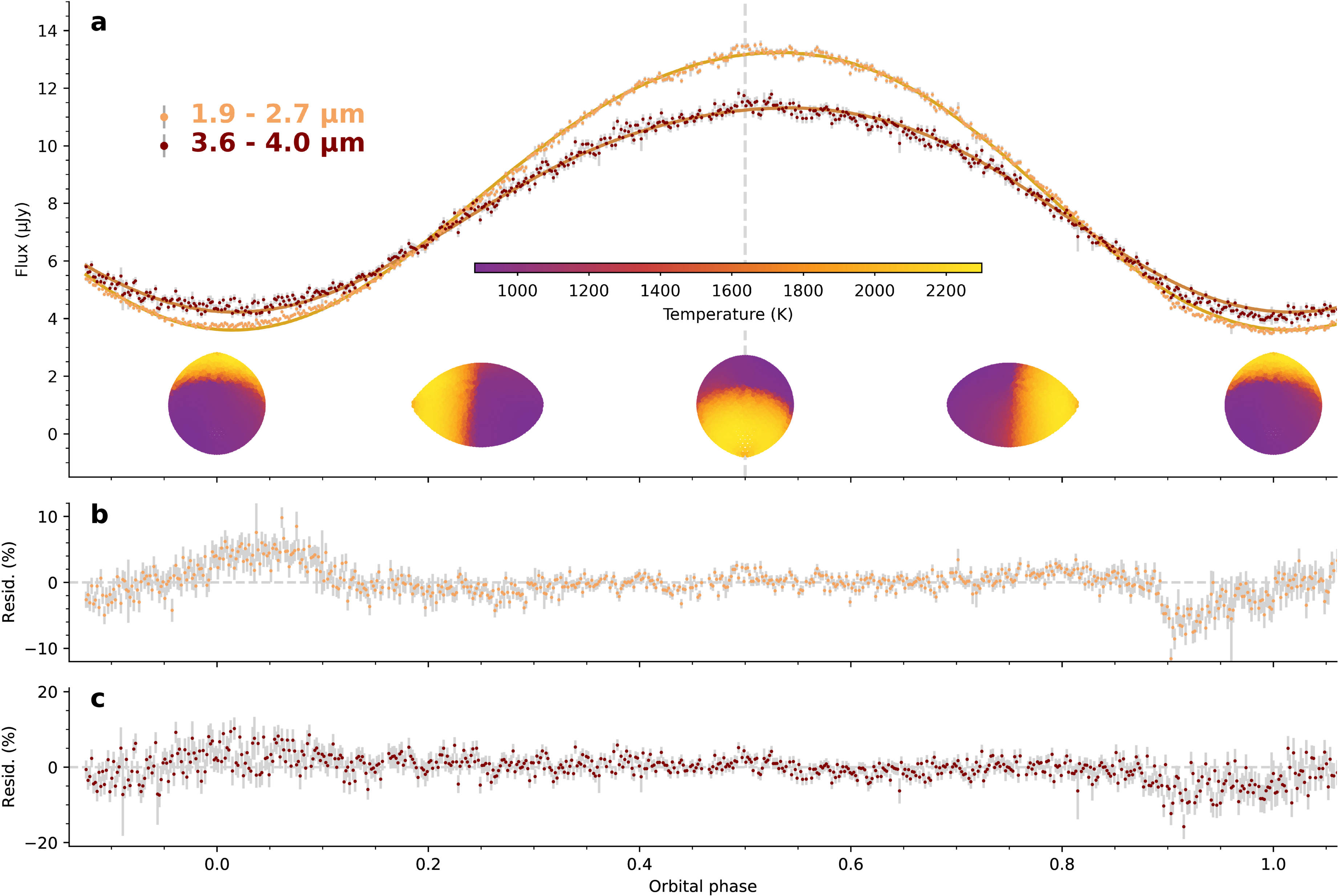
Next, we model the PRISM phase curve. The C3 absorption depth varies dramatically with orbital phase, complicating modeling of the heated companion surface. However, at wavelengths of relatively low opacity, a basic thermal model can be used to constrain the binary properties. Figure 5 shows the light curves in two wavelength ranges between the strongest absorption bands. The flux varies by ∼three times from day to night, a modest amplitude compared to other black-widow companions, which can show modulations of 30–100 times (P. Draghis et al. 2019). The light curves exhibit nightside variability—the second minimum is 10% lower than the first, possibly due to flares (D. Kandel & R. W. Romani 2020). We model the light curves in the two opacity windows by assuming Planckian emergent spectra and direct pulsar heating, using a version of the ICARUS heated binary light-curve code (R. P. Breton et al. 2012; see Section 5). All fits require a near-filled Roche lobe. Fitting the full light curves, we find i ∼ 31∘, with photosphere temperatures ranging from 900 K at the coldest points on the nightside to 2300 K at the hottest points on the dayside. We infer a distance consistent with the radio parallax measurement and a westward wind. Given the closeness of the inferred inclination to the values we obtained previously by assuming reasonable pulsar masses, it is not surprising that we now infer a pulsar mass (∼2.0M⊙ with 0.1 M⊙ statistical error and 0.5M⊙ systematic error) consistent with astrophysical expectations (see Appendix 5). The inferred isotropic heating luminosity of 9 × 1032 erg s−1 is 5/I45 times the pulsar’s spindown luminosity, where 1045I45 g cm2 is the pulsar’s moment of inertia. The apparent over-unity heating efficiency is an artifact of the pulsar’s gamma-ray emission being beamed along the spin equator (and, hence, toward the companion), possibly in combination with a large moment of inertia arising from a high pulsar mass.
Figure 5. The companion light curve in two continuum bands interpreted with a pulsar direct heating model. (a) The models are shown by the curves and the data are shown by the points. The model does not capture the strong orbit-to-orbit variations at minimum (ϕ ∼ 0 and ϕ ∼ 1) but provides a good description of the flux from the heated face and constrains the binary parameters (see Section 5). Schematics of the Earth view of the heated companion’s surface temperature are shown below the light curve. (b) and (c) The residuals of the models compared to their corresponding light curves.
Download figure:
Standard image High-resolution image 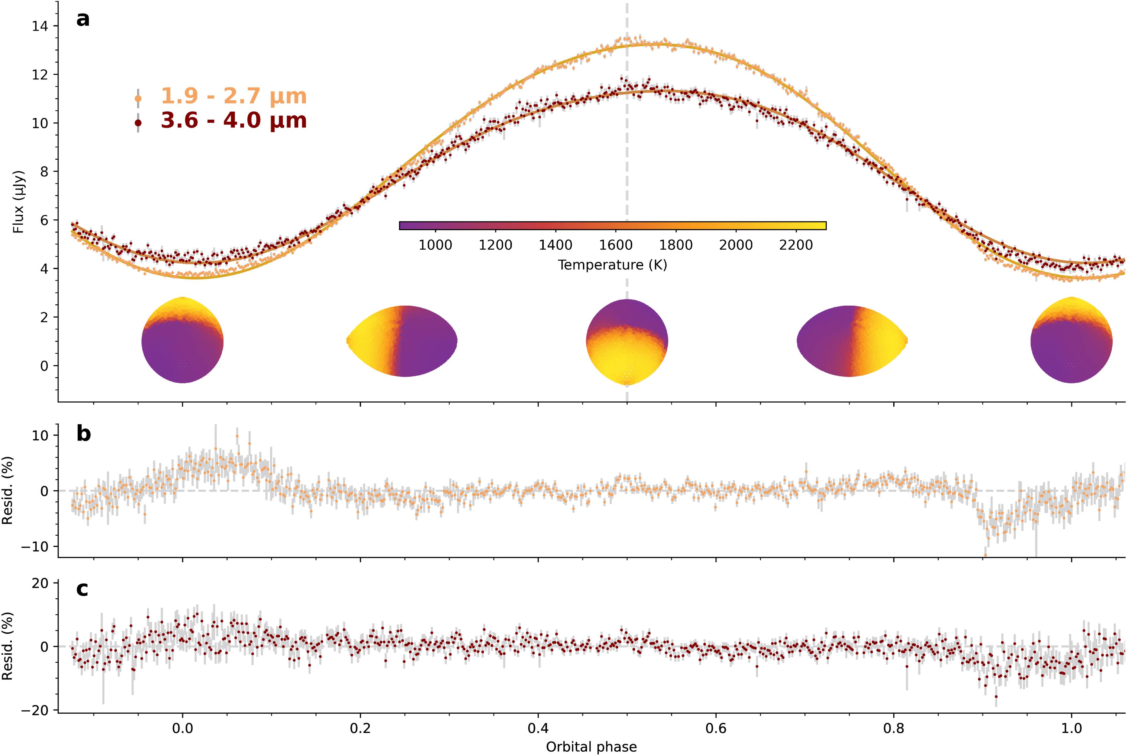
The flux maximum in the phase curve occurs 12∘ after phase 0.5, indicating a westward offset that is suggestive of strong winds blowing opposite to the planet’s rotation direction. A westward thermal phase offset is seen in some black-widow companions (D. Kandel & R. W. Romani 2020) and is rare among hot Jupiters orbiting main-sequence stars (T. J. Bell et al. 2021), having only been robustly observed for CoRoT-2b (L. Dang et al. 2018). All of these objects have rotation periods equal to their orbital periods, due to tidal locking, but PSR J2322–2650b’s exceptionally short rotation period of 0.32 days places it in a different dynamical regime from almost all hot Jupiters. E. K. H. Lee et al. (2020) and X. Tan & A. P. Showman (2020) demonstrated with 3D general circulation models (GCMs) that, at very short rotation periods of ≲10 hr, the equatorial eastward jet ubiquitous on slower-rotating hot Jupiters narrows, while off-equatorial westward zonal winds become increasingly distinctive, leading to a westward phase offset. Because we do not expect the dynamics on PSR J2322–2650b to be identical to X. Tan & A. P. Showman (2020), due to the very different form of irradiation, we run a planet-specific atmospheric dynamics model with MITgcm (see Appendix E). Our temperature maps are qualitatively similar to theirs; in particular, we also obtain a westward phase offset. Our data are therefore observational evidence of the dynamical regime that X. Tan & A. P. Showman (2020) predicted—a regime rarely probed by hot Jupiters orbiting main-sequence stars.
Better line lists and improvements in the modeling of planetary atmospheres will allow more accurate computation of inclination and pulsar mass through modeling of the spectroscopic phase curve. This could be particularly interesting for PSR J2322–2650, because the pulsar’s low intrinsic spindown  implies an exceptionally low neutron star dipole field 2.5 × 10⁷I45 G. This is relevant, since the reduced magnetic field of millisecond pulsars is often attributed to accretion during the spinup process (G. S. Bisnovatyi-Kogan & B. V. Komberg 1974; R. E. Taam & E. P. J. van den Heuvel 1986; R. W. Romani 1990; D. Mukherjee 2017); with such a low field, the pulsar may have accreted a large amount of matter, achieving a larger moment of inertia and a high mass. Thus, precise measurement of the masses in this system could help constrain MTOV, the Tolman–Oppenheimer–Volkoff mass, which sets the maximum mass for a slowly rotating neutron star and constrains the dense matter equation of state.
Our findings pose a challenge to the current understanding of black-widow formation, in which a pulsar strips the outer layers of its stellar companion by a combination of Roche-lobe overflow and photoevaporation (O. G. Benvenuto et al. 2012; Y. Guo et al. 2022). This mechanism can produce a helium-dominated Jupiter-mass object if stripping occurs before core helium burning, during the main sequence or red giant branch. In this picture, these black widows are the descendants of ultracompact X-ray binaries with He-star donors, and the core C/N/O ratios can be sensitive to the evolutionary state of the donor at the start of Roche-lobe overflow (see Figure 4 of G. Nelemans et al. 2010). How this process produces a C/O ratio greater than 100 or a C/N ratio greater than 10,000 is difficult to explain. Although G. Nelemans et al. (2010) predict extreme N depletion in one scenario (see their Figure 4, bottom middle), O becomes significantly enhanced relative to C in this scenario. In the other two scenarios (corresponding to different initial helium-star masses), C is enhanced relative to O by a factor of ∼15, but it is only enhanced relative to N by a factor of ∼several. Although extreme photospheric ratios are possible via gravitational settling for the much-higher-gravity white dwarfs (the immediate progenitors of black-widow companions in the standard formation scenario), gravitational settling is not expected to differentiate elements once the companion becomes a planetary mass object with a molecular atmosphere.
Other mechanisms of carbon enrichment pose their own challenges. For example, the helium-dominated, hydrogen-poor, and carbon-enriched composition of PSR J2322–2650b is reminiscent of R Coronae Borealis (RCB) stars and dustless hydrogen-deficient carbon (dLHdC) stars, which are believed to result from mergers of He and CO white dwarfs (R. F. Webbink 1984; H. Saio & C. S. Jeffery 2002). However, the rarity of RCB/dLHdC stars and the necessity of invoking three stars makes them unlikely progenitors, and the measured C/O and C/N ratios of these stars (12–81 and 4–130, respectively; A. Mehla et al. 2025) are still lower than the very high minimum values we obtain. The triple-alpha process, which fuses helium into carbon, creates asymptotic giant branch “carbon stars” with C/O ratios of up to ∼several (C. Abia et al. 2008) but not the C/O > 100 inferred from our data. Carbon stars have a dusty outflow rich in carbon grains (M. Di Criscienzo et al. 2013), providing a further source of carbon enrichment, but further modeling is required to explain how this carbon ultimately ends up in a Jupiter-mass object. More spectroscopic observations of ultralow-mass black-widow companions (“Tidarrens”) are needed to determine whether PSR J2322–2650b’s composition is unusual or representative of the class. We particularly encourage observations of PSR J1719–1438, which has a similar mass but a far higher minimum density of 21 g cm−3, leading M. Bailes et al. (2011) to suggest it is an ultralow-mass carbon white dwarf.
A Jupyter notebook is available to reproduce the figures in this work in Zenodo (M. Zhang 2025) at doi:10.5281/zenodo.17400581. The repository also includes the spectra plotted in Figure 2(a) in ASCII format.
The authors thank Gerald Kerley for providing the carbon equation of state used for the interior structure models. T.D.K. acknowledges Jayne Birkby, Luke Parker, and Stephen Smartt for insightful discussions. M.Z. thanks Qiao Xue, Keeyoon Sung, Sergey Yurchenko, John Tonry, and Jeremy Goodman for insightful feedback. M.B. thanks Jaikhomba Singha and Andrea Possenti for comments on the pulsar timing section and Sarah Buchner for observing. P.G. acknowledges Shazrene Mohamed and Mikako Matsuura for enlightening discussions.
These observations are associated with JWST GO #5263 and the work is funded by the associated grant. The MeerKAT telescope is operated by the South African Radio Astronomy Observatory, which is a facility of the National Research Foundation, an agency of the Department of Science and Innovation. M.Z. acknowledges support from the 51 Pegasi b Fellowship funded by the Heising–Simons Foundation. Part of this work was undertaken for the Australian Research Council Centre of Excellence for Gravitational Wave Discovery (project number CE230100016). Support for this work was provided by NASA through the NASA Hubble Fellowship grant HST-HF2-51559.001-A awarded by the Space Telescope Science Institute, which is operated by the Association of Universities for Research in Astronomy, Inc., for NASA, under contract NAS5-26555.
M.Z. proposed the observations, led the project, identified C3 and C2, and led the writing of the Letter. M.B. fit the continuum light curves with ICARUS to obtain temperature maps and constrain binary parameters. T.D.B. performed the data analysis using primarily custom software. R.W.R. gave advice on the pulsar physics, proposed a plausible formation mechanism, and helped with light-curve fitting. P.G. searched opacity databases to identify spectral features and ran atmospheric forward models to fit the spectrum. H.B. ran, postprocessed, and interpreted GCMs with a bespoke heating scheme. M.B. is the PI of the MeerTime Large Survey Project, oversees the pulsar portal/pipeline, and created the standard profile, arrival times, and initial model fits. M.N. performed the interior structure calculations. J.L.B. helped conceive the project and gave advice through all stages. T.D.K. helped with GCM development and interpretation and writing the manuscript. B.P.C. suggested the identification of C–H spectral features. G.F. performed an independent data reduction. R.L. helped with the figures and with data interpretation. D.J.R. conducted pulsar timing analysis to determine system parameters. E.C. ran and maintained the pipeline producing the MeerKAT pulsar timing data. R.M.S. is the PI of the MeerKAT PTA timing project and conducted pulsar timing analysis to determine system parameters. J.J.F. advised on the interior structure and atmosphere modeling. A.A.A.P. performed a blackbody retrieval and gave comments on the manuscript. M.C.M. edited the Letter and contributed to understanding the pulsar heating. J-M.D. contributed to the proposal.
Facilities: JWST - James Webb Space Telescope (NIRSpec), MeerKAT - .
Software: astropy (Astropy Collaboration et al. 2013, 2018, 2022), JWST Calibration Pipeline (H. Bushouse et al. 2025), HELIOS (M. Malik et al. 2017, 2019), HELIOS-K (S. L. Grimm et al. 2021), FastChem (J. W. Stock et al. 2022).
The distance to the pulsar is important for the interpretation of this system in at least two ways: it determines the luminosity of the companion, and it allows us to derive the intrinsic spindown rate  , due to the Shklovskii correction for pseudo-acceleration (I. S. Shklovskii 1970). The pulsar’s spindown luminosity and inferred magnetic field strength are both related to
  . The PSR J2322–2650 discovery paper (R. Spiewak et al. 2017) reported a low timing parallax distance of
  pc, much smaller than their dispersion measure (DM) model distance of 760 pc. M. Shamohammadi et al. (2024), using the more accurate MeerKAT radio telescope data set, obtained a timing parallax of 1.3 ± 0.2 mas, from which was derived a distance of 770
 pc. Here, we improve the distance estimate by extending the MeerKAT data set.
The 3.46 ms pulsar J2322–2650 is observed regularly as part of the MeerKAT Pulsar Timing Array (MPTA; M. T. Miles et al. 2023), using the PTUSE pulsar instrument (M. Bailes et al. 2020). Observations span from 2019 July to 2025 April, and we obtain arrival times at 136 different epochs in 16 coherently dispersed frequency subbands, spanning 775.0 MHz centered at 1283.582 MHz. A standard pulse profile is created by aligning all data with the optimal DM and with the phase-connected timing solution, removing the dispersion and averaging into 16 subbands, before wavelet smoothing with the psrchive (W. van Straten et al. 2012) application psrsmooth. Topocentric arrival times are measured with a standard Fourier-domain pulse profile cross-correlation technique, with uncertainties estimated with a Monte Carlo simulation. Arrival times with a signal-to-noise ratio of cross-correlation below 10 are removed, and we perform a least-squares fit using tempo2 (G. B. Hobbs et al. 2006) for the pulsar spin, binary, and astrometric parameters on the 2625 remaining arrival times. The reduced χ2 is 1.0, and the weighted rms and median residuals are 2.2 μs and 3.4 μs, respectively, indicating a good model fit.
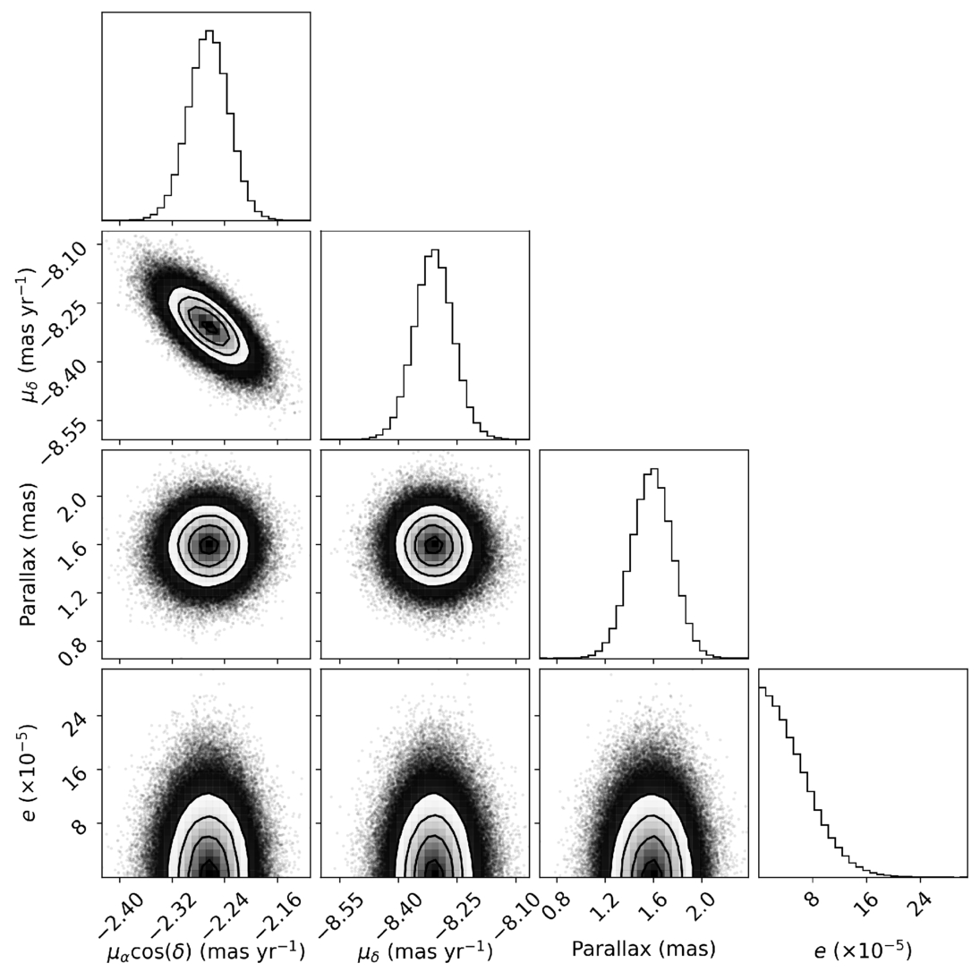
We infer posterior probability distributions for the timing model parameters together with noise parameters using the Bayesian pulsar timing package inference enterprise (J. A. Ellis et al. 2020). We use a noise model that is standard in pulsar timing array analyses (including for the MPTA; M. T. Miles et al. 2025), which describes white noise, DM variations, and achromatic red noise in timing residuals. However, no significant red-noise processes were detected. Corner plots (D. Foreman-Mackey 2016) of the 1D and 2D marginal posterior probability distributions for the main timing model parameters of interest are shown in Figure 6. The measured timing model parameters are provided in Table 1, including the pulsar parallax, proper motion, period, and period derivative. We do not detect orbital eccentricity and place a 95% upper limit of e < 0.00012. The pulsar distance derived from the parallax is  pc and the transverse velocity with respect to the Sun is just 26 km s−1. Correcting for the peculiar motion of the Sun means that the velocity of the pulsar is small in the local standard of rest and indistinguishable from random motions in the Galaxy. The pulsar is experiencing Shklovskii pseudo-acceleration due to its transverse velocity and distance, and this implies that the intrinsic period derivative is
  , where μ is the pulsar proper motion and c is the speed of light. Such a low period derivative makes PSR J2322–2650 one of the pulsars with the weakest magnetic field strengths known (
 ), which may have helped the planet survive irradiation from the pulsar.
Figure 6. Posterior probability distributions for key pulsar parameters from the timing of PSR J2322–2650 with the MeerKAT radio telescope.
Download figure:
Standard image High-resolution image 
Table 1. Measured Timing Parameters of PSR J2322–2650
ParameterValue
Pulsar Parameters
R.A., α (J2000)23:22:34.638364(4)
decl., δ (J2000)−26:50:58.39619(8)
Proper motion in R.A.,  −2.26(3) mas yr−1
Proper motion in decl., μ**δ−8.31(5) mas yr−1
Spin period (P)3.463099179266747(4) ms
Period derivative (
−2.26(3) mas yr−1
Proper motion in decl., μ**δ−8.31(5) mas yr−1
Spin period (P)3.463099179266747(4) ms
Period derivative ( )5.8586(16) × 10−22 s s−1
Epoch (MJD)59693.0
DM6.14449(4) pc cm−3
Parallax1.59(17) mas
Semimajor axisa 0.00278444 (s)
Orbital period0.3229640004(7) days
Eccentricity, e<0.00012 (95%)
MJD ascending node59692.9699957(14)
Derived Parameters
)5.8586(16) × 10−22 s s−1
Epoch (MJD)59693.0
DM6.14449(4) pc cm−3
Parallax1.59(17) mas
Semimajor axisa 0.00278444 (s)
Orbital period0.3229640004(7) days
Eccentricity, e<0.00012 (95%)
MJD ascending node59692.9699957(14)
Derived Parameters
Distance, D  pc
Transverse velocity26 ± 3 km s−1
Intrinsic
pc
Transverse velocity26 ± 3 km s−1
Intrinsic  1.8(4) × 10−22
Note. aProjected semimajor axis of the pulsar (not the companion), in light-seconds.
Download table as: ASCIITypeset image
We extract 1D spectra from the uncalibrated JWST data using a mixture of the JWST pipeline and our own software and methods. The first stage of the pipeline consists of fitting a count rate to each pixel’s measured sequence of accumulated counts. While we follow the general approach of the JWST pipeline, we use our own software for every step of this stage. Some of the changes in our approach have since been implemented in the official pipeline.
Correlated 1/f noise (S. H. Moseley et al. 2010) is typically corrected by the JWST pipeline using non-light-sensitive reference pixels. Unfortunately, our data are in subarray mode, where most of these reference pixels are skipped rather than being read out. Our treatment of 1/f noise differs somewhat from that of the JWST pipeline. We describe that approach first, as we use it for all of our data processing, including the construction of dark reference files.
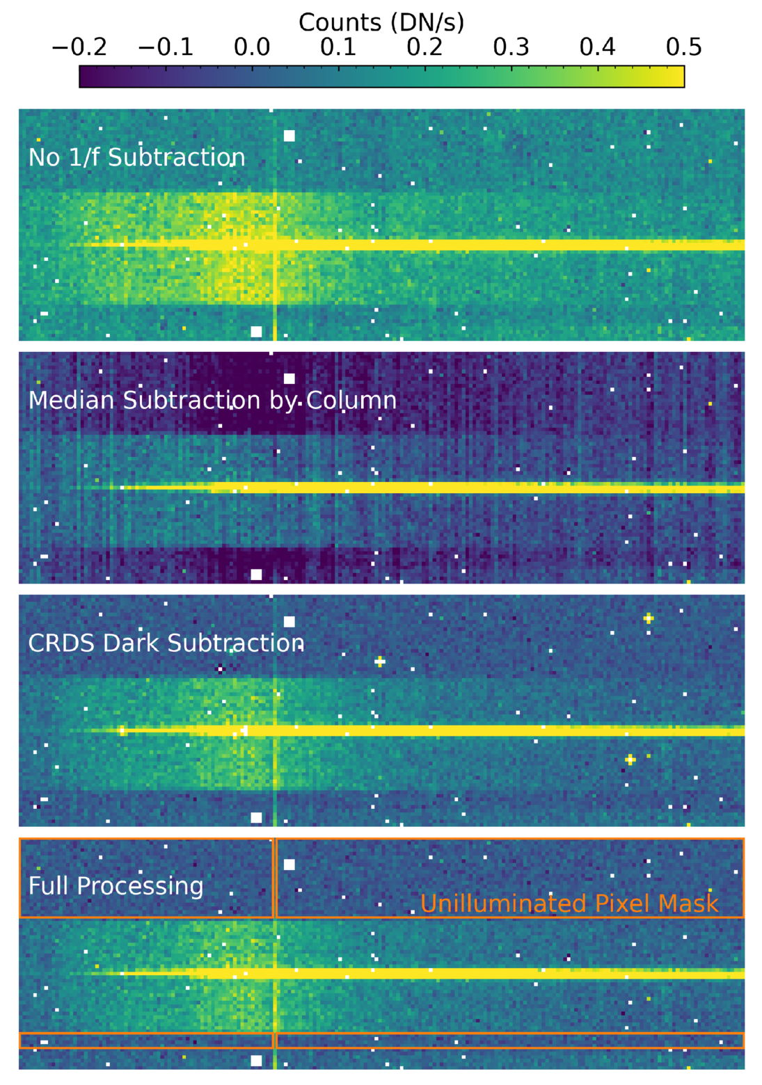
The 1/f noise is correlated in time. The pixels in the NIRSPEC subarrays are read out in columns, with each pixel in a column being read out sequentially, before moving on to the next column. As a result, temporally correlated noise appears as a spatial correlation, with the value of the noise being similar among all pixels in a column. There are several approaches that can be used to mitigate this 1/f noise. One is to compute and subtract the median value column by column from each read, while another is to determine a set of pixels that receive no signal (or nearly no signal) and to use these to construct a noise model. Figure 7 shows both of these approaches, together with the result of doing no correction, in the top three panels. In each case, we show the count rate averaged over the same 10 integrations with the same linear color scale.
Figure 7. Comparison of different data reduction processes for the PRISM data, averaged over 10 integrations. The region shown encompasses just under half of the full PRISM spectrum.
Download figure:
Standard image High-resolution image 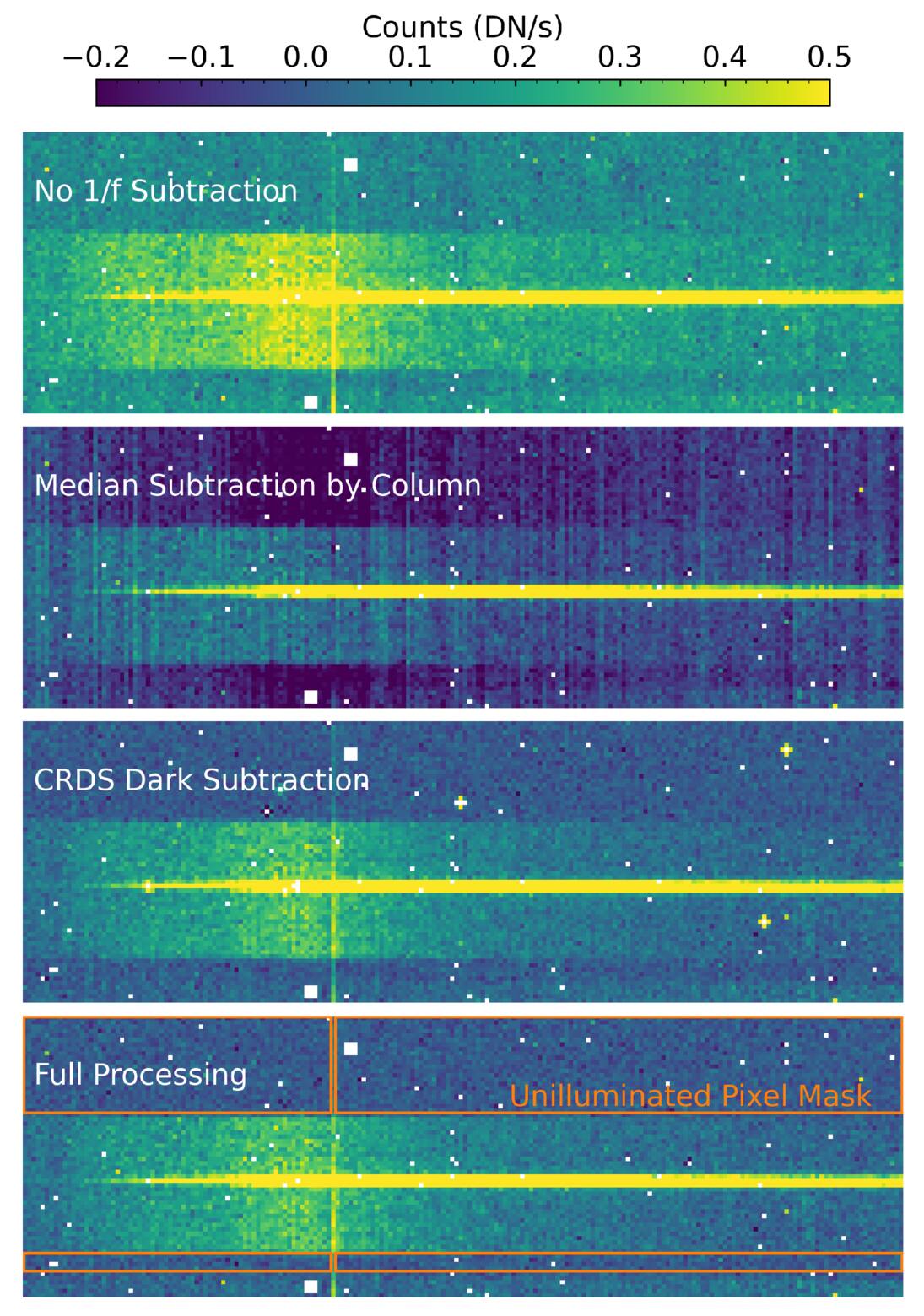
The top panel of Figure 7 shows the result with no 1/f correction. The background regions have a visibly nonzero count rate, due to the low-frequency component of the 1/f that is shared by all reads; it would have a different value if a different set of integrations were averaged together. The second panel shows the result of a median subtraction column by column. It shows large single-column deviations from systematically different pixels along with biases from the fact that science data are not excluded.
Our 1/f noise correction, shown in the third and fourth panels of Figure 7, is based on the NSClean algorithm (B. J. Rauscher 2024) as implemented in the JWST pipeline (H. Bushouse et al. 2025). Our changes to the algorithm consist of tuning the frequencies to be corrected and designing a custom mask for the pixels to be used. For PRISM data, we use four rows (numbers 7–10 of 64, beginning from 1) between shutters, in addition to the top 22 rows. These rows (with the exception of one bad column) are shown in the bottom panel of Figure 7. The frequencies to be corrected are specified by four numbers. Frequencies below the lowest number or above the highest number (in Hz) are not corrected; frequencies between the second and third numbers are fully fit. Frequencies between the first and second numbers, and between the third and fourth numbers, are apodized—i.e., fit with a weight that smoothly varies between 0 and 1. The default values for these four frequencies are 1061, 1211, 49,943, and 49,957 Hz. The latter number is just below 50,000 Hz; odd–even noise appears at a frequency of half the pixel rate of 100 kHz and is corrected. We adopt values of 200, 600, 49,943, and 49,957 for our correction frequencies—i.e., we fit for lower-frequency noise than the pipeline defaults. We are able to do this because we have more pixels available for fitting in our custom mask than in the default mask.
In addition to the 1/f correction, we also revisit the JWST pipeline step of the dark subtraction. The dark signal and bad pixels available at the JWST Calibration Reference Data System (CRDS)18 have evolved since those data were taken and do not provide a perfect match to our data. Further, the dark signal for most pixels is extremely small, so that it is measured by the dark reference files only with low signal-to-noise ratios. As a result, we do not perform a dark subtraction for most pixels. Any dark that we would construct or use from CRDS would have a realization of read noise in it, even if this read noise is averaged over many integrations. Our mean spectra are themselves averaged over nearly 700 integrations, so the dark could easily make a significant contribution to the total read noise. To avoid adding unnecessary read noise, we use darks only to correct the neighbors of hot pixels.
We define hot pixels for our purposes as those that accumulate more than 250 counts in 30 reads. We do not aim to recover the value of the hot pixel but simply to remove the impact it makes on its neighbors due to interpixel capacitance. To get this right pixel by pixel for our PRISM data, we construct a dark image for each read, from 151 integrations of grating data with the same subarray configuration. These data do have a faint visible trace. We fit this trace with a quadratic in pixel coordinates. Near the trace, the grating-derived dark would be an inappropriate choice, as it is not truly dark. We therefore substitute the value of the CRDS dark for pixels within 3 pixels of the center of the grating trace.
Finally, we use our hybrid dark to correct hot pixels and their immediate neighbors, before masking the hot pixels themselves. For an isolated hot pixel, we scale the dark to the science frame and subtract it in a 3 × 3 patch around the hot pixel. The hot pixel itself now has zero flux; we mask it for all further analysis. The immediate neighbors of the hot pixel now have had the effects of interpixel capacitance removed. If a hot pixel is not isolated, we need to be careful not to doubly remove the interpixel capacitance. We use the same algorithm described above, but for pixels that border more than one hot pixel, we split their values across multiple 3 × 3 patches. The bottom panel of Figure 7 shows the impact of the hot-pixel processing, with neighbors of hot pixels appearing to be consistent with the large-scale background.
The steps above create a calibrated set of individual reads, but we still must fit for a count rate for each pixel in each integration. For this, we use the likelihood-based ramp-fitting and jump-detection algorithms described in T. D. Brandt (2024a) and T. D. Brandt (2024b). These were integrated into the JWST pipeline after these data were reduced. So-called snowballs (M. Regan 2024) are clusters of pixels showing a jump in counts after an ene