[TOC]

INTRODUCTION

The survival of our species owes much to our brain, specifically, its ability to observe, analyse, and plan. Planting crops and storing grains for the winter were some of the earliest uses of these abilities. Measuring and calculating are foundational elements of observation, analysis, and planning. Computation, upon which our modern society depends, is but an extension of those ancient measurement and calculation techniques.

Calculations operate on operands obtained through measurements. Counting was the oldest form of measurement. In prehistory, humans counted by scratching marks on bones. Next to evolve was a ruler etched with markings. Thereafter, humans were marking, measuring, calculating, tracking, and predicting the movements of the Sun and the Moon using stone pillars, astronomically aligned burial mounds, and sun dials.

By around 3000 BC, Sumerians invented the sexagesimal (base-$60$) number system, and they were using the abacus by 2700 BC. The abacus was one of the earliest devices that mechanised calculations, and it is still in extensive use, throughout the world. A cuneiform clay tablet from 1800 BC shows that Babylonians already knew how to survey land boundaries with the aid of Pythagorean triples. Egyptians improved upon these techniques to survey property boundaries on the Nile flood planes and to erect the pyramids. By 220 BC, Persian astronomers were using the astrolabe to calculate the latitude, to measure the height of objects, and to triangulate positions. Greeks constructed truly advanced mechanical instruments that predicted solar and lunar eclipses. The sophistication and refinement exhibited by the Antikythera mechanism from around 200 BC continues to amaze modern engineers.

Ancient astronomy measured, tracked, and predicted the movements of heavenly objects. But when celestial navigation came to be used extensively in global trade across the oceans, we began charting the night sky in earnest, and thus was born modern astronomy. Astronomical calculations involved manually manipulating numbers. Those calculations were tedious and error prone.

In 1614, a brilliant Scottish mathematician John Napier discovered logarithms. Perhaps it would be more appropriate to say Napier invented logarithms, for his discovery was motivated by his desire to simplify multiplication and division. Arithmetically, multiplication can be expressed as repeated additions, and division as repeated subtractions. Logarithmically, multiplication of two numbers can be reduced to addition of their logarithms, and division to subtraction thereof. Hence, multiplication and division of very large numbers can be reduced to straightforward addition and subtraction, with the aid of prepared logarithm and inverse logarithm tables.

In 1620, Edmund Gunter, an English astronomer, used Napier’s logarithms to fashion a calculating device that came to be known as Gunter’s scale. The markings on this device were not linear like a simple ruler, but logarithmic. To multiply two numbers, the length representing the multiplicand is first marked out on the logarithmic scale using a divider and, from thence, the length representing the multiplier is similarly marked out, thereby obtaining the product, which is the sum of the two logarithmic lengths. Gunter’s scale mechanised the tedious task of looking up numbers on logarithm tables. This device was the forerunner of the slide rule.

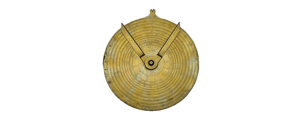
The first practical slide rule was invented by William Oughtred, an English mathematician, in 1622. Oughtred used two bits of wood graduated with Gunter’s scale to perform multiplication and addition. Then, in 1630, Oughtred fashioned a brass circular slide rule with two integrated pointers. This device was a significant improvement over Gunter’s scale, in terms of practicality and usability. The photograph below shows a brass circular slide rule that is a contemporaneous clone of Oughtred’s.

The earliest adopters of the slide rule were the 17th century astronomers, who used it to perform arithmetic and trigonometric operations, quickly. But it was the 19th century engineers, the spearheads of the Industrial Revolution, who propelled the slide rule technology forward. For nearly four centuries after its invention, the slide rule remained the preeminent calculating device. Buildings, bridges, machines, and even computer system components, were designed by slide rule. Apollo astronauts carried the Pickett N600-ES pocket slide rule, onboard, for navigation and propulsion calculations. The General Dynamics F-16, a modern, air-superiority fighter, was designed by slide rule. Well into the late 1970s, school children all over the world, including me, were taught to use the slide rule and the logarithm book, along with penmanship and grammar.

The largest and most enthusiastic group of slide rule users, naturally, were engineers. But slide rules were used in all areas of human endeavour that required calculation: business, construction, manufacturing, medicine, photography, and more. Obviously, bankers and accountants relied on the slide rule to perform sundry arithmetic gymnastics. Construction sites and factory floors, too, used specialised versions of slide rules for mixing concrete, computing volumes, etc. Surveyors used the stadia slide rule made specifically for them. Doctors use special, medical slide rules for calculating all manner of things: body mass index, pregnancy terms, medicine dosage, and the like. Photographers used photometric slide rules for calculating film development times. Army officers used artillery slide rules to compute firing solutions in the field. Pilots used aviation slide rules for navigation and fuel-burn calculations. The list was long. This humble device elevated the 18th century astronomy, powered the 19th century Industrial Revolution, and seeded the 20th century Technological Revolution. Indeed, the slide rule perfectly expressed the engineering design philosophy: capability through simplicity.

But then, in 1972, HP released its first programmable scientific calculator, the inimitable HP-35. The HP-35 rang loud the death knell of the slide rule. Although electronic pocket calculators were unaffordable in the early 1970s, they became ubiquitous within a decade thanks to Moore’s law and Dennard’s law, and quickly displaced the slide rule. By the early 1980s, only a few people in the world were using the slide rule. I was one.

personal

It was around this time that I arrived at the university—in Burma. In those days, electronic pocket calculators were beyond the reach of most Burmese college students. To ensure fairness, my engineering college insisted that all students used the government-issued slide rule, which was readily accessible to everyone. Many classrooms in my college had large, wall-mounted demonstration slide rules to teach first-year students how properly to use the slide rule like an engineer—that is, to eradicate the bad habits learned in high school. As engineering students, we carried the slide rule upon our person, daily.

I subsequently emigrated to the US. Arrival in the US ended my association with the slide rule because, by the 1980s, American engineers were already using HP RPN pocket calculators and MATLAB technical computing software on the IBM PC. I soon became an HP calculator devotee. As such, I never got to use the slide rule extensively in a professional setting. But I hung on to my student slide rules: the government-issued Aristo 0968 Studio, a straight rule, and the handed-down Faber-Castell 8/10, a circular rule. To this day, I remain partial to the intimate, tactile nature of the slide rule, especially the demands it places upon the user’s mind. Over the next four decades, I collected many slide rules, dribs and drabs. The models in my collection are the ones I admired as an engineering student in Burma, but were, then, beyond reach.

In its heyday, everyone used the slide rule in every facet of life. As children, we saw it being used everywhere, so we were acquainted with it, even if we did not know how to use it. We were taught to use the slide rule’s basic facilities in middle school. Our options were the abacus, the log books, or the slide rule. The choice was abundantly clear: we enthusiastically took up the slide rule—a rite of passage, as it were. Now, though, even the brightest engineering students in the world have never heard of a slide rule, let alone know how it works.

goal

My main goal in writing this article is to preserve the knowledge about, and the memory of, this ingenious computing device: how it works and how it was used. The focus here is on the basic principles of operation and how the slide rule was used in engineering. This is a “how it works” explanation, and not a “how to use” manual. Those who are interested in the most efficient use of a slide rule may read the manuals listed in the resources section at the end of this article. Beyond history and reminiscence, I hope to highlight the wide-ranging utility of some of the most basic mathematical functions that are familiar to middle schoolers.

recommendations

It is mighty difficult to discuss the slide rule without having the device in hand. For the presentations below, I chose the Keuffel & Esser (K&E) 4081-3 Log Log Duplex Decitrig, a well-made wood rule. It was one of the most popular engineering slide rules for decades, especially in the US. As such, many engineering professors published good introductory books for it, and these books are now available online in PDF format.

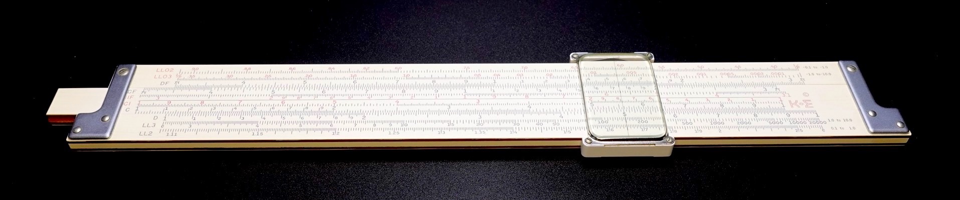
The term “log-log” refers to the $LL$ scale, which is used to compute exponentiation, as will be explained, later. The term “duplex” refers to the fact that both sides of the frame are engraved with scales, a K&E invention. The label “Decitrig” was K&E’s trade name for its slide rules that used decimal degrees for trigonometric computations, instead of minutes and seconds. Engineers prefer using the more convenient decimal notation.

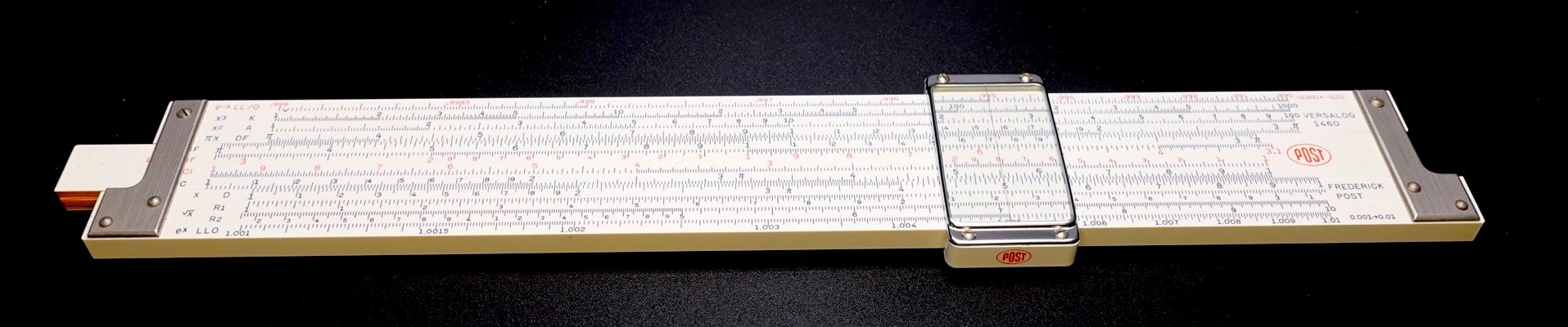
Another common model was the Post 1460 Versalog. Although less popular than the K&E 4081-3, the Post 1460 is cheaper and, in my opinion, is a better slide rule. It is made of bamboo, a more stable material than wood.

Go on eBay and buy a good, inexpensive slide rule, either the K&E 4081-3 or the Post 1460; you will need a slide rule to follow the discussions below. Alternatively, you could use a slide rule simulator. The feature of this simulator that is especially useful to novices is the cursor’s ability instantaneously to show the exact scale values under the hairline.

And I recommend that, after you have read this article, you study one or more of the books listed in the resources section at the end.

PRINCIPLES

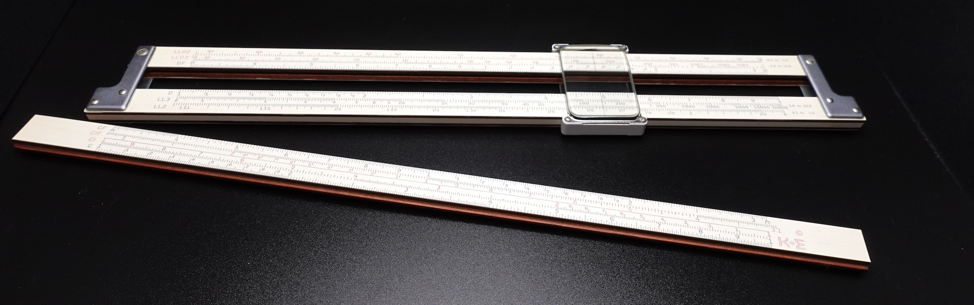
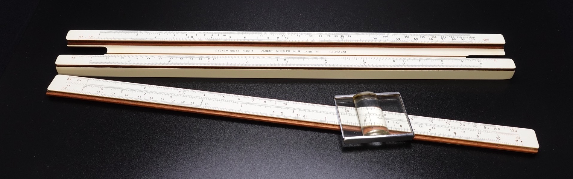
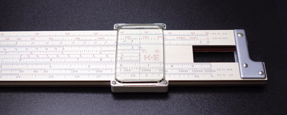
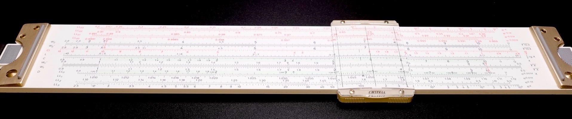
A slide rule comprises three components: the body, the slide, and the cursor, as shown below. The body, about 25 cm in length, consists of two pieces of wood, the upper and the lower frames, bound together with metal brackets at the ends. The slide is a thin strip of wood that glides left and right between the upper and the lower frames. The cursor consists of two small plates of glass held by metal brackets and these brackets are anchored to the upper and the lower lintels. The cursor straddles the body and glides across its length. Hence, the three components of a slide rule move independently of, and with respect to, one another.

A duplex slide rule, like the K&E 4081-3 shown below, both sides of the frame have scales, and so do both sides of the slide. These scales are set and read using the hairline inscribed on the cursor glass. The cursor cannot slip off the body, because it is blocked by the metal brackets at the ends of the body.

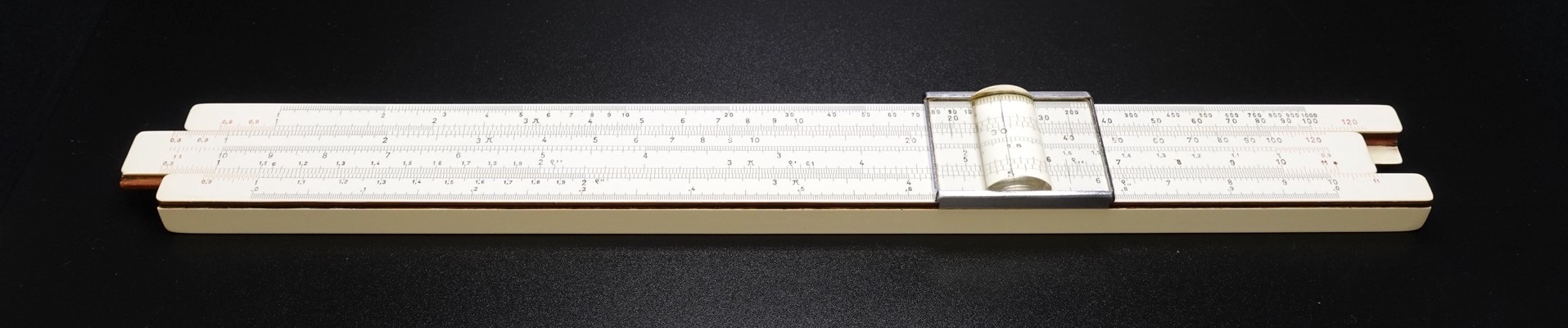
A simplex slide rule, like the Nestler 23 R shown below, the cursor can slip off the body. The body is a single piece of wood with a trough in the middle separating the upper and the lower frames. Only the frontside of the frame has scales, but the slide has scales on both sides.

The slide rule is always operated using both hands, fingers of one hand pushing and those of the other gently opposing. The lower lintel of the cursor glides along the bottom of the lower frame. There is a tension spring between the upper lintel of the cursor and the top of the upper frame. This tension spring braces the lower lintel of the cursor flush against the bottom of the lower frame. To make fine adjustments of the cursor, one uses the thumbs of both hands against the lower lintel of the cursor. It is important to avoid touching the upper lintel, since it does not sit flush against the frame, due to the tension spring. When using the backside of a duplex straight rule, the lower lintel of the cursor has now flipped to the topside, so it had to be fine adjusted using the forefingers. Fine adjustments of the slide are made with the thumb or the forefinger of one hand opposing its counterpart of the other hand. To use the backside scales on a duplex straight rule, the device is flipped bottom-to-top.

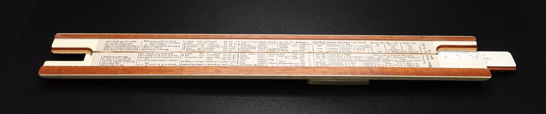
Simplex slide rules have use instructions and a few scientific constants on the back, but duplex slide rules come with plastic inserts that bear such information. But no engineer I knew actually used this on-device information. Procedures for operating an engineering slide rule are complex; we had to study the user’s manual thoroughly and receive hands-on instructions for several weeks before we became proficient enough to be left alone with a slide rule without causing mayhem in the laboratory. And every branch of engineering has its own set of published handbooks in which many formulae and constants can readily be found.

arithmetic operations

properties of logarithms—The base-$10$ common logarithm function $log(x)$ and its inverse, the power-of-10 function $10^x$, give life to the slide rule. The two main properties of logarithms upon which the slide rule relies are these:

$$ \begin{align} a × b &= log^{-1}[log(a) + log(b)] \nonumber \ a ÷ b &= log^{-1}[log(a) - log(b)] \nonumber \end{align} $$

That is, to compute $a × b$, we first compute the sum of $log(a)$ and $log(b)$, then compute the $log^{-1}$ of the sum. Likewise, $a ÷ b$ is computed as the $log^{-1}$ of the difference between $log(a)$ and $log(b)$.

logarithmic scale—The slide rule mechanises these calculations by using two identical logarithmic scales, commonly labelled $C$ (on the slide) and $D$ (on the frame). Gunter’s logarithmic scale is derived from a ruler-like linear scale in the following manner. We begin with a 25-cm-long blank strip of wood and mark it up with $10$ equally spaced segments labelled $0, 1, 2, 3, …, 10$, similar to an ordinary ruler, but labelling the ending $10$ as $1$, instead. This first piece of wood has now become the source linear scale. We then line up the second 25-cm long blank strip of wood with the first one, and mark up that second piece of wood with $9$ unequally spaced segments labelled $1, 2, 3, …, 1$, starting with $1$ and, again, ending with $1$. The division marks of the second piece of wood is placed non-linearly in accordance with their $log$ values and by reference to the linear scale:

• $log(1) = 0.0$, so $1$ on the non-linear scale is lined up with $0.0$ on the linear scale
• $log(2) = 0.301$, so $2$ on the non-linear scale is lined up with $0.301$ on the linear scale
• $log(3) = 0.477$, so $3$ on the non-linear scale is lined up with $0.477$ on the linear scale
• $…$
• $log(10) = 1.0$, so $10$ (which is labelled $1$) on the non-linear scale is lined up with $1.0$ on the linear scale

The second scale thus obtained is the non-linear, logarithmic scale. In the figure below, the upper one is the source linear scale and the lower one is the derived logarithmic scale.

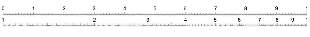
On the slide rule, the source linear scale is labelled $L$, and it is called the “logarithm scale”. The derived logarithmic scale is labelled $D$.

I would like to direct your attention to this potentially confusing terminology. The term “logarithm scale” refers to the linear $L$ scale used for computing the common logarithm function $log(x)$. And the term “logarithmic scale” refers to the non-linear $C$ and $D$ scales used for computing the arithmetic operations $×$ and $÷$. This knotty terminology is unavoidable, given the logarithmic nature of the slide rule.

The logarithmic scale and the logarithm scale are related by a bijective function $log$:

$$ \begin{align} log &: D \rightarrow L \nonumber \ log^{-1} &: L \rightarrow D \nonumber \end{align} $$

In the plot below, the black curve is $log$ and the red is $log^{-1}$.

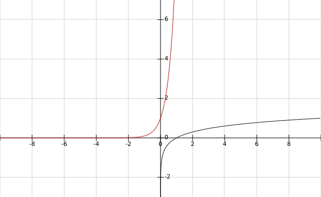
The special name for $log^{-1}$ is power-of-$10$ function $10^x$. The $D$ and the $L$ scales form a transform pair that converts between the logarithmic scale and the arithmetic scale. It turns out that the $log$ function transforms the arithmetic scale’s $×$ and $÷$ operators into the logarithmic scale’s $+$ and $-$ operators, and the $log^{-1}$ function performs the inverse transformation.

Plotting the $log$ function on a logarithmic scale produces a sequence of evenly spaced values. Hence, the $L$ scale appears linear, when laid out on the slide rule. Note also that the mere act of reading $x$ on the logarithmic scale implicitly computes $log(x)$; there is no need explicitly to compute $log^{-1}(x)$. Gunter’s logarithmic scale was the groundbreaking idea that made the slide rule work so effectively, efficiently, effortlessly.

The logarithmic scale has many other uses in STEM beyond the slide rule: the Richter scale used to measure seismic events; the $dB$ decibel scale used to measure sound pressure levels; the spectrogram used to visualise frequency domain signals are just a few examples. These uses exploit the logarithms’ ability to compress a very large range, while preserving relevant details.

computations using logarithmic scales—To compute $2 × 3$, we manipulate the slide rule as follows:

1. $D$—Place the hairline on the multiplicand $2$ on the $D$ scale.
2. $C$—Slide the left-hand $1$ on the $C$ scale under the hairline.
3. $C$—Place the hairline on the multiplier $3$ on the $C$ scale.
4. $D$—Read under the hairline the product $6$ on the $D$ scale. This computes $2 × 3 = 6$.

The above multiplication procedure computes $2 × 3 = 6$, like this:

• In step (1), we placed the hairline on $D$ scale’s $2$. In this way, we mechanically marked out the length $[1, 2]$ along the logarithmic $D$ scale. Mathematically, this is equivalent to computing $log(2)$.
• In step (2), we lined up $C$ scale’s left-hand $1$, the beginning of the scale, with $D$ scale’s $2$, in preparation for the next step.
• In step (3), we placed the hairline on $C$ scale’s $3$. This mechanically marked out the length sum $[1, 2]_D + [1, 3]_C = [1, 6]_D$ on the logarithmic $D$ scale, which is mathematically equivalent to computing $log(2) + log(3) = log(6)$.
• Then, in step (4), we read the result $6$ on the $D$ scale under the hairline. This is mathematically equivalent to computing $log^{-1}[log(2) + log(3)] = 2 × 3 = 6$. Recall that $log^{-1}$ operation is implicit in the mere reading of the $D$ logarithmic scale.

To put it another way, adding $2$ units of length and $3$ units of length yields $2 + 3 = 5$ units of length on the arithmetic scale of an ordinary rule. But on the logarithmic scale of the slide rule, adding $2$ units of length and $3$ units of length yields $2 × 3 = 6$ units of length.

To compute $2 ÷ 3$, we manipulate the slide rule as follows:

1. $D$—Place the hairline on the dividend $2$ on the $D$ scale. This computes $log(2)$.
2. $C$—Slide under the hairline the divisor $3$ on the $C$ scale.
3. $C$—Place the hairline on the right-hand $1$ on the $C$ scale. This computes $log(2) - log(3) = log(0.667)$.
4. $D$—Read under the hairline the quotient $667$ on the $D$ scale, which is interpreted to be $0.667$, as will be explained in the next subsection. This computes $2 ÷ 3 = log^{-1}[log(2) - log(3)] = 0.667$.

Multiplication and division operations start and end with the cursor hairline on the $D$ scale. Skilled users frequently skipped the initial cursor setting when multiplying and the final cursor setting when dividing, opting instead to use the either end of the $C$ scale as the substitute hairline.

accuracy and precision

In slide rule parlance, accuracy refers to how consistently the device operates—that is, how well it was manufactured and how finely it was calibrated. And precision means how many significant figures the user can reliably read off the scale.

Professional-grade slide rules are made exceedingly well, so they are very accurate. Yet, they all allow the user to calibrate the device. Even a well-made slide rule, like the K&E 4081-3 can go out of alignment if mistreated, say by exposing it to sun, solvent, or shock (mechanical or thermal). Misaligned slide rule can be recalibrated using the procedure described in the maintenance section, later in this article. And prolonged exposure to moisture and heat can deform a wood rule, like the K&E 4081-3, thereby damaging it, permanently. The accuracy of a warped wood rule can no longer be restored by recalibrating. So, be kind to your slide rule.

To analyse the precision of the slide rule, we must examine the resolution of the logarithmic scale, first. The $C$ and $D$ scales are logarithmic, so they are nonlinear. The scales start on the left at $log(1) = 0$, which is marked as $1$, and end on the right at $log(10) = 1$, which is also marked as $1$. Indeed, these scales wrap around by multiples of $10$ and, hence, the $1$ mark at both ends.

As can be seen in the figure below, the distance between two adjacent major divisions on the scale shrinks logarithmically from left to right:

• $log(2) - log(1) = 0.301 \approx 30%$
• $log(3) - log(2) = 0.176 \approx 18%$
• $log(4) - log(3) = 0.125 \approx 12%$
• $log(5) - log(4) = 0.097 \approx 10%$
• $log(6) - log(5) = 0.079 \approx 8%$
• $log(7) - log(6) = 0.067 \approx 7%$
• $log(8) - log(7) = 0.058 \approx 6%$
• $log(9) - log(8) = 0.051 \approx 5%$
• $log(10) - log(9) = 0.046 \approx 4%$

The figure above also shows the three distinct regions on the $D$ scale that have different resolutions:

• In the range $[1, 2]$, the scale is graduated into $10$ major divisions, and each major division is further graduated into $10$ minor divisions.
• In the range $[2, 4]$, the scale is graduated into $10$ major divisions, and each major division is further graduated into $5$ minor divisions.
• In the range $[4, 1]$, the scale is graduated into $10$ major divisions, and each major division is further graduated into $2$ minor divisions.

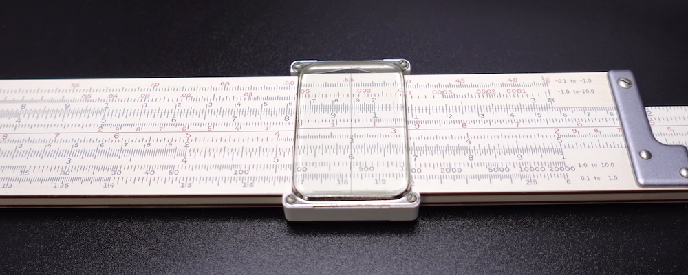
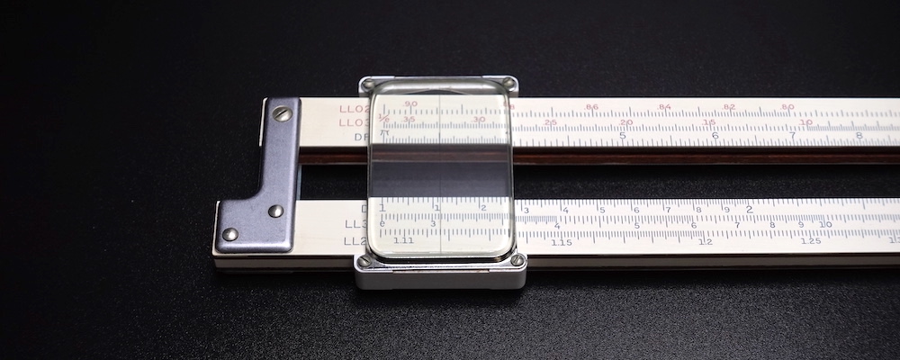
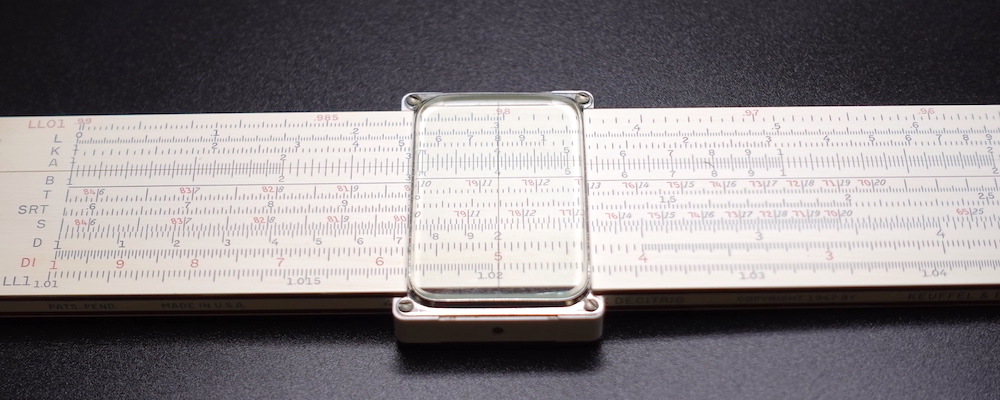
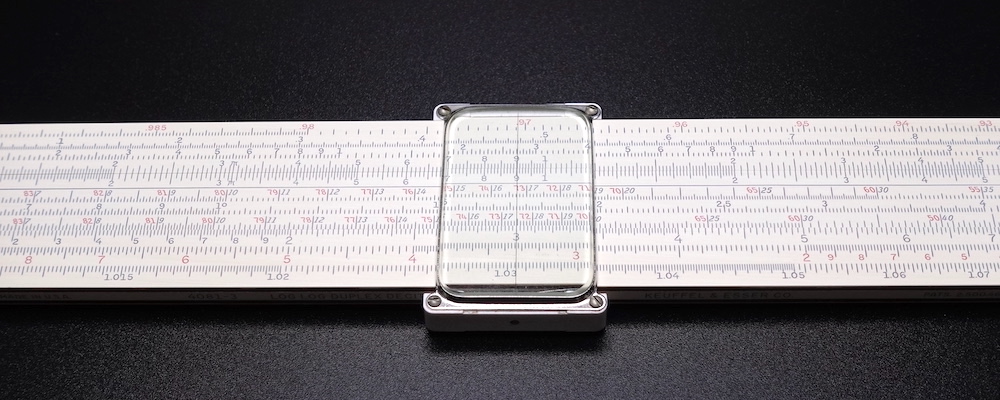
At the left end of the $D$ scale, $1.11$, $1.12$, etc., can be read directly from the scale. With practice, one could visually subdivide each minor division into $10$ sub-subdivisions and discern $1.111$ from $1.112$, reliably, precisely. In the photograph below, the cursor hairline is placed on $1.115$.

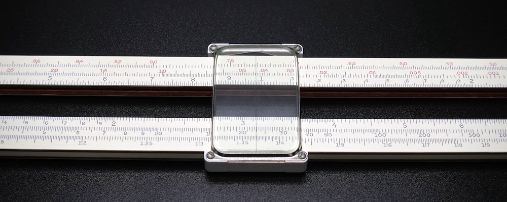
In the middle of the $D$ scale, $3.12$, $3.14$, etc., can be read directly from the scale. Indeed, $3.14$ is marked as $\pi$ on $C$ and $D$ scales of all slide rules. With a nominal eyesight, each minor division could be subdivided visually and easily read $3.13$, which is halfway between the $3.12$ and the $3.14$ graduations. The photograph below shows the hairline on $3.13$.

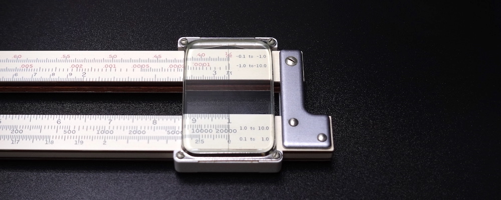
On the right end of $D$ scale, $9.8$, $8.85$, $9.9$, $9.95$, etc., can be read directly from the scale. With due care, each minor division could be subdivided into two sub-subdivisions and read without undue strain $9.975$, which is halfway between the $9.95$ and the $1$ graduations. See the photograph below. But for those of us with poor eyesights, it is rather difficult to discern $9.98$ from $9.99$.

Under optimal conditions—calibrated slide rule, nominal eyesight, good lighting, and alert mind—the slide rule can attain four significant figures of precision on the lower end of the $D$ scale and three significant figures on the higher end of the scale.

It is important to note that the logarithmic scale cycles, repeatedly. Hence, the scale reading of $314$ can be valued as $…$, $0.0314$, $0.314$, $3.14$, $31.4$, $314.0$, $3140.0$, $…$ and so forth, depending on the context. The decimal point must be located using mental arithmetic. For example, $\pi/8 \approx 3/8 \approx 0.4$, so the result must necessarily be $0.3927$, not $0.03927$, $3.927,$ nor anything else. So, mental arithmetic locates the decimal point thereby getting us within the zone of accuracy, and scale reading yields the constituent digits thus getting us the precision we desire.

Ordinarily, the slide rule was used to evaluate complicated expressions involving many chained calculations when they needed to be performed quickly, but when precision was not a paramount concern. When precision is important, however, logarithm tables were used. These tables were laboriously hand-computed to several significant figures. If the desired value fell between two entries in the table, the user is obliged to interpolate the result, manually. While actuaries may have demanded the high precision afforded by the logarithm table, engineers willingly accepted three or four significant figures offered by the slide rule, because the slide rule was accurate enough for engineering use and it was the fastest means then available to perform calculations. In due course, the slide rule became inextricably linked to engineers, like the stethoscope to doctors.

It might be shocking to a modern reader to learn that slide rule wielding engineers accepted low-precision results, considering how precise today’s engineering is, owing to the use of computer-aided design (CAD) and other automation tools. But these high-tech tools came into common use in engineering, only in the 1990s. Before that, we had to perform analysis by hand using calculators, and prior to that with slide rules. In fact, engineering analysis was a tedious affair. For instance, to design a simple truss bridge—the kind prevalent in the 19th century—the structural engineer must compute the tension and compression forces present in each beam, taking into account the dimensions of the beams, the strengths of various materials, expected dynamic loads, projected maximum winds, and many other factors. The analysis of force vectors involves many arithmetic and trigonometric calculations, even for the simplest of structures. The sheer number calculations made it uneconomical to insist upon the higher precisions offered by the logarithm tables. As such, engineers settled for lower precision, and in compensation incorporated ample safety margins. This was one of the reasons why older structures are heftier, stronger, and longer-lasting, compared to their modern counterparts.

VARIETIES

Slide rules came in straight, circular, and cylindrical varieties. Cylindrical rules consist of two concentric cylinders that slide and rotate relative to each other. The key innovation of cylindrical rules was the helical scale that wraps round the cylinder. This coiled scale stretches to an impressive length, despite the relatively small size of the cylinder. Of course, a longer scale yields a greater precision. The cylinder can be rotated to bring the back-facing numbers round to the front.

Circular rules were the first practical slide rules. Their main advantages are compactness and stoutness. A typical model is constructed like a pocket watch and operated like one too, using crowns. The glass-faced, sealed construction protects the device against dust. Some circular models sport a spiral scale, thereby extracting good precision from a compact real estate. But the circular scales oblige the user to rotate the device frequently for proper reading. Expert users of circular rules were good at reading the scales upside-down. On some very small models, the graduation marks get very tight near the centre. In other words, circular rules can be rather fiddly.

Of all the varieties, straight rules are the easiest and the most convenient to use, because they are relatively small and light, and because the whole scale is visible at once. However, their scale lengths are bounded by the length of the body. So, straight rules are less precise by comparison.

Most engineers preferred straight rules, because these devices allowed the user to see the whole scales, and they were fast, accurate, and portable enough for routine use. Hence, this article focuses on straight rules. But a few engineers did use circular models, either because these devices were more precise or because they were more compact. In general, engineers did not use cylindrical ones; these devices were too unwieldy and they had only basic arithmetic scales. But accountants, financiers, actuaries, and others who required greater precision swore by cylindrical rules.

straight rules

The commonest kind of slide rule was the 25 cm desk model, called the straight rule. The cursor is made of clear plastic or glass, etched with a hairline. The frame and the slide are made of wood, bamboo, aluminium, or plastic. The name “slide rule” derives from the slippy-slidy bits and the ruler-like scales. Straight rules come in four types: Mannheim, Rietz, Darmstadt, and log-log duplex.

The less expensive Mannheim and Rietz models were used in high school, and the more sophisticated Darmstadt and log-log duplex models were used in college. There were longer straight rules used by those who required more precision. And there were shorter, pocket-sized straight rules, like the Pickett N600-ES carried by the Apollo astronauts. Although not very precise, pocket slide rules were good enough for quick, back-of-the-napkin calculations in the field. Engineers, however, were partial to the 25 cm desk straight rule. As such, the majority of the slide rules manufactured over the past two centuries were of this design.

Mannheim type—The most basic straight rule is the Mannheim type, the progenitor of the modern slide rule. Surely, applying the adjective “modern” to a device that had been deemed outmoded for over 40 years is doing gentle violence to the English language. But given that the slide rule is now over 400 years old, a 150-year-old Mannheim model is comparatively “modern”.

A Mannheim slide rule has $C$ and $D$ scales for arithmetic operations ($×$ and $÷$), $L$ scale for common logarithm ($log$), $A$ and $B$ scales for square and square root ($x^2$ and $\sqrt{x}$), $K$ scale for cubic and cube root ($x^3$ and $\sqrt[3]{x}$), and $S$ and $T$ scales for trigonometric functions ($sin$ and $tan$).

The following is the Post 1447 simplex slide rule, manufactured by the Japanese company Hemmi in the late 1950s. As is the tradition for Japanese slide rules, this one is made of bamboo, which is a better material than wood, because bamboo is more resistant to warping and it slides more smoothly. The term “simplex” refers to the slide rules with scales on only one side of the frame.

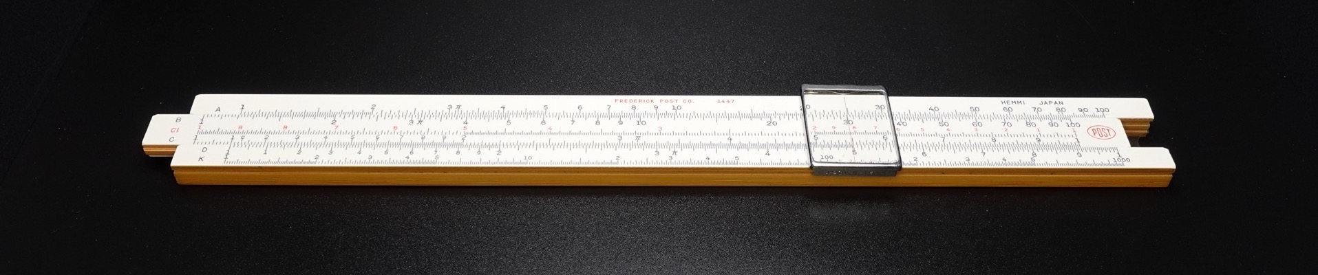
Unlike its simplex frame, the slide of the Mannheim rule has engraved on its backside the $S$, $L$, and $T$ scales, which are read through the cutouts at each end. Given that the Post 1447 is a modern Mannheim rule, it has clear-plastic windows over the cutouts, and engraved on these windows are fixed red hairlines for reading the scales. These hairlines are alined with the $1$ mark on the frontside $D$ scale.

Classic Mannheim simplex slide rules do not have windows over the cutouts. Instead, their cutouts are cleverly placed in an offset: the right-hand cutout is aligned with the two upper scales on the backside of the slide (the $S$ and the $L$ scales) and the left-hand cutout is aligned with the two lower scales (the $L$ and the $T$ scales). It does get unwieldy when trying to read the left-edge of the $S$ scale, but this design compromise significantly reduces the need to flip the slide round to the front. If the predominant calculations are trigonometric, however, it is more convenient to just flip the slide and to use the front of the slide rule.

The original Mannheim slide rule was invented in 1859 by Amédée Mannheim, a French artillery officer, for quickly computing firing solutions in the field. It had only $C$, $D$, $A$, and $B$ scales, so it was capable of computing only $×$, $÷$, $x^2$, and $\sqrt{x}$. This suited its intended purpose. It was the forefather of the modern straight rule.

Rietz type—A slight improvement upon the French Mannheim type was the German Rietz type, designed in 1902 for Dennert & Pape (D&P, subsequently Aristo) by Max Rietz, an engineer. It added the $ST$ scale for small angles in the range $[0.573°, $ $5.73°] = [0.01, 0.1]\ rad$. In this angular range, $sin(\theta) \approx tan(\theta)$, so the combined $sin$-$tan$ scale suffices. The following is the Nestler 23 R Rietz, a German make known to be favoured by boffins, including Albert Einstein. The 23 R dates to 1907, but the example below is from the 1930s. The frontside has $K$ and $A$ scales on the upper frame; $B$, $CI$ , and $C$ scales on the slide; and $D$ and $L$ scales on the lower frame. The $CI$ scale is the reverse $C$ scale that runs from right to left.

The backside of the Nestler 23 R have traditional, Mannheim-style offset cutouts at each end and black index marks engraved onto the wood frame. The backside of the slide holds the $S$, $ST$, and $T$ scales. The $S$ and $ST$ scales are read in the right-hand cutout, and the $ST$ and the $T$ scales are read in the left-hand cutout.

Some slide rules, like this older Nestler 23 R below, came with magnifying cursor glass to allow a more precise scale reading. But I find the distorted view at the edges of the magnifier rather vexing. This model looks to be from the 1920s.

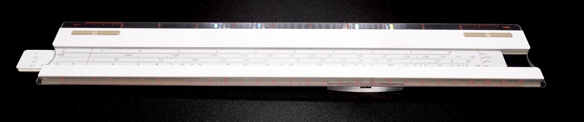
Darmstadt type—Another German innovation was the Darmstadt type, designed in 1924 by Alwin Walther, a professor at the Technical University of Darmstadt, for D&P (Aristo). Darmstadt rule was the workhorse preferred by the early 20th century engineers. It added three $LL_n$ scales ($LL_1$, $LL_2$, and $LL_3$) which are used to compute general exponentiation of the form $x^{y/z} = \sqrt[z]{x^y}$, when $x > 1$. When $z = 1$, the general expression reduces to $x^y$. When $y = 1$, the general expression reduces to $x^{1/z} = \sqrt[z]{x}$. Newer, more advanced models sport the fourth $LL_0$ scale. The following is the Aristo 967 U Darmstadt from the mid 1970s.

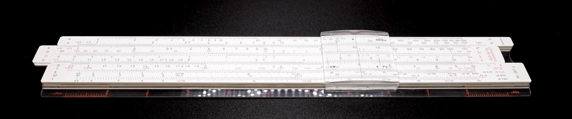
The backside of the Aristo 967 U’s slide has the $L$ and the three $LL_n$ scales. Being that it is a late model Darmstadt simplex rule with a clear plastic back, the entire lengths of these scales are visible at once—a definite improvement to usability compared to the tradition wood rules with cutouts. These scales are read against the fixed red hairline at each end.

log-log duplex type—Modern engineering slide rules generally are of the log-log duplex type. The duplex scale layout was invented by William Cox in 1895 for K&E. The models used by engineering students have three black $LL_n$ scales ($LL_1$, $LL_2$, and $LL_3$ running from left to right) for cases where $x > 1$ and three red $LL_{0n}$ scales ($LL_{01}$, $LL_{02}$, and $LL_{03}$ running from right to left) for cases where $x < 1$. More advanced models used by professional engineers have four black-red pairs of $LL$ scales.

The Faber-Castell (FC) 2/83 N Novo Duplex slide rule, shown below, is a late model, advanced engineering rule from the mid 1970s. It was designed and manufactured at the close of the slide rule era. It was especially popular outside the US. It is a rather long and wide slide rule. And it was arguably one of the most aesthetically pleasing slide rules ever made.

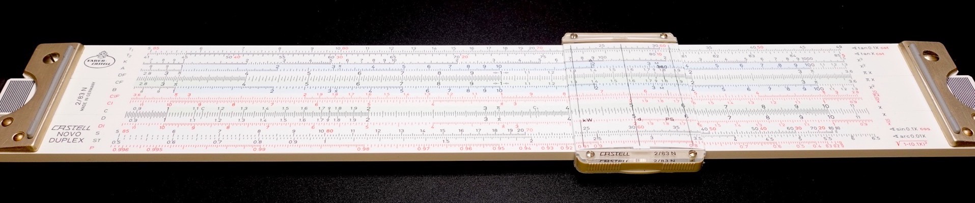
Aside from sporting four black-red pairs of $LL$ scales on the backside, the FC 2/83 N has $T_1, T_2$ expanded $tan$ scales and $W_1, W_2$ specialised scale pairs for computing $\sqrt{x}$ with greater precision.

circular rules

Circular slide rules can be categorised into three types: simplex, pocket watch, and duplex. Circular rules were popular with businessmen, and the most popular models were of the stylish, pocket watch type.

simplex type—The diameter of the FC 8/10 circular rule is only 12 cm, but in terms of capability, it is equivalent to a 25-cm Rietz straight rule. The FC 8/10 is an atypical circular rule: most circular rules use spiral scales, but the FC 8/10 uses traditional Rietz scales in wrapped, circular form. The example shown below was made in the mid 1970s.

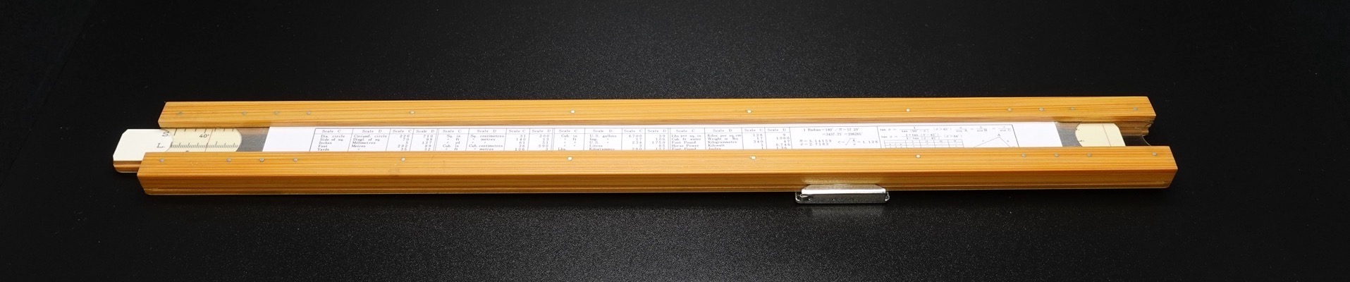
Since the FC 8/10 is a simplex circular rule, its backside holds no scales; instead it bears use instructions and a few scientific constants.

pocket watch type—A more typical design for circular slide rules is the pocket watch variety, like the Fowler’s Universal Calculator shown below. William Fowler of Manchester, England, began manufacturing calculating devices in 1898. This particular model probably dates to the 1950s. Fowler slide rules were made to exacting standards, like a stylish, expensive pocket watch, and are operated like a watch, too, using the two crowns.

The backside of the Fowler’s Universal Calculator is covered in black leather. This device is small enough to fit in the palm and the edges of the metal case are rounded, so it is quite comfortable to hold.

duplex type—It is no secret that most engineers disliked the circular slide rule; many were downright derisive. Seymour Cray, the designer of the CRAY super computer, my favourite electrical engineer and my fellow circular slide rule fancier, once quipped, “If you had a circular [slide rule], you had some social problems in college.” But the Dempster RotaRule Model AA was the circular rule that even the most ardent straight rule enthusiast found tempting. It is a duplex circular rule. And it is exceedingly well made. Its plastic is as good as the European plastics, far superior to the plastics used by American manufacturers like K&E. It is the brainchild of John Dempster, an American mechanical engineer. The Dempster RotaRule Model AA shown below is probably from the late 1940s. Unconventionally, the trigonometric scales are on the frontside.

The backside of the Dempster RotaRule holds the four $LL_n$ scales among others.

cylindrical rules

All cylindrical rules emphasise precision, so they all have very long scales. Some cylindrical rules use the helical-scale design, while others use the stacked straight-scale design. Cylindrical rules come in two types: pocket type and desk type. The business community favoured the greater precision these devices afforded. As such, most cylindrical rules were very large; they were made for the banker’s ornate mahogany desk.

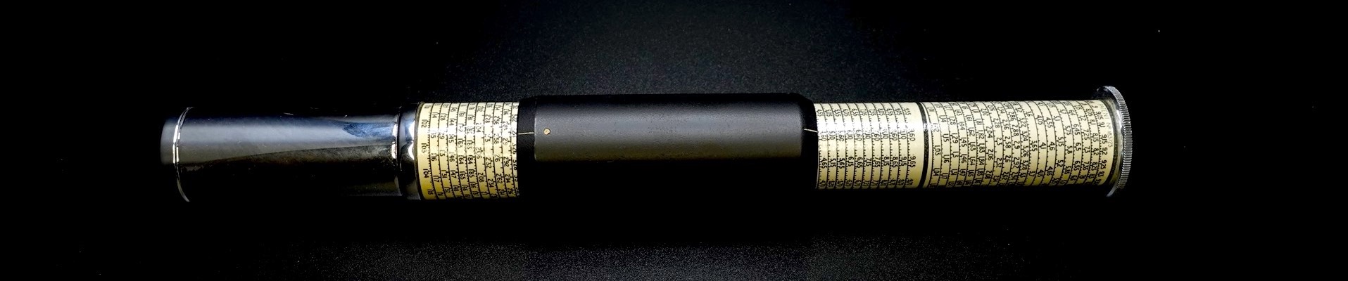
pocket type—The Otis King Model L, shown below, is a contradiction: it is a compact cylindrical rule that, when collapsed, is well shy of an open palm. Portability wise, this cylindrical rule could compete with larger pocket watch type circular rules. But because the Model L employs helical scales, its precision is far superior to that of common straight rules and pocket watch circular rules. This particular Model L is likely from the 1950s.

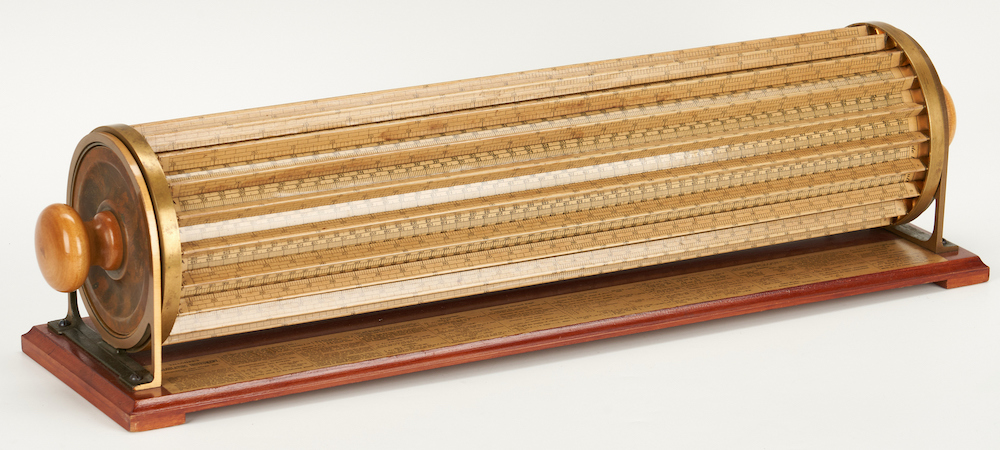
desk type—A giant among large cylindrical rules was the K&E 1740, designed in 1881 by Edwin Thacher, an American engineer working for K&E. I have never seen this device in person, so I do not know the finer points of how it was used. But the general operating principles are similar to that of the Otis King Model K: the outer cylinder is mounted to the wooden base but it can spin in place. The inner cylinder shifts and spins independently of the outer cylinder. The inner cylinder’s scale is read through the slits in the outer cylinder’s scale. Thus, the outer cylinder is analogous to the straight rule’s frame, and the inner cylinder is analogous to the straight rule’s slide. There is, however, no cursor on this device; it is unnecessary, since the large, legible scales can be lined up against each other by eye. The first Thacher model dates to 1881. The one shown in the photograph blow, a museum piece, is probably a late model from the 1950s, by the look of it.

OPERATIONS

Ordinary engineering slide rules provide arithmetic, logarithm, exponential, and trigonometric functions. Some advanced models provide hyperbolic functions. More models provide speciality-specific functions: electronic, electrical, mechanical, chemical, civil, and so forth. Here, I shall ignore such speciality-specific rules.

arithmetic

The impetus for the slide rule’s invention was to expedite $×$ and $÷$. These arithmetic operations were performed using the $C$ and the $D$ scales. Over time, slide rule designers had created numerous scales that augment the $C$ and $D$ scales: reciprocal $CI$ and $DI$; folded $CF$ and $DF$; and folded reciprocal $CIF$ and $DIF$.

In 1775, Thomas Everard, an English excise officer, inverted Gunter’s logarithmic scale, thus paving the way for the reciprocal $CI$ and $DI$ scales that run from right to left. Using $D$ and $C$, $a ÷ b$ is computed as $a_D - b_C$. But using $D$ and $CI$, this expression is computed as $a_D + b_{CI}$:

$$ \begin{align} a ÷ b &= log^{-1}[log(a) - log(b)] \nonumber \ &= log^{-1}[log(a) + log(\frac{1}{b})] \nonumber \end{align} $$

The $CF$, $DF$, $CIF$, and $DIF$ scales are called “folded”, because they fold the $C$, $D$, $CI$, and $DI$ scales, respectively, at $\pi$, thereby shifting the $1$ mark to the middle of the scale. The following photograph shows these auxiliary scales on the slide.

These auxiliary scales often reduce slide and cursor movement distances considerably, thereby speeding up computations. But I shall not present the detailed procedures on using these auxiliary scales, because they are procedural optimisations not essential to understanding slide rule fundamentals. Interested readers may refer to the user’s manuals, which are listed in the resource section at the end of the article.

logarithm

The logarithm $L$ scale is the irony of the slide rule. The $log$ function is nonlinear. But because the slide rule is based upon this very same nonlinearity, the $L$ scale appears linear when inscribed on the slide rule.

To compute $log(2)$, we manipulate the slide rule as follows:

1. $D$—Place the cursor hairline on the argument $2$ on the $D$ scale.
2. $L$—Read under the hairline the result $0.301$ on the $L$ scale. This computes $log(2) = 0.301$.

exponentiation

squaring on slide rule—A typical engineering slide rule provides the $A$ scale on the frame and the $B$ scale on the slide for computing $x^2$, the $K$ scale on the frame for computing $x^3$, and the $LL_n$ scales and their reciprocals $LL_{0n}$ scales on the frame for computing $x^y$. The procedures for computing powers and roots always involve the $D$ scale on the frame.

To compute $3^2$, we manipulate the slide rule as follows:

• $D$—Place the hairline on the argument $3$ on the $D$ scale.
• $A$—Read under the hairline the result $9$ on the $A$ scale. This computes $3^2 = 9$.

The $A$-$D$ scale pair computes $x^2$, because $A$ is a double-cycle logarithmic scale and $D$ is a single-cycle logarithmic scale. In the reverse direction, t