1748-9326/20/11/114063

Abstract

Luxury crops such as grapes, coffee, and cacao have immense economic and cultural importance in many regions. Climate change is affecting growing conditions across the globe. Natural climate variability may exacerbate the impact of increasing temperature and shifting precipitation patterns, leading to large interannual variations in yields, potentially resulting in revenue loss. Stratospheric aerosol injection (SAI), a form of solar climate intervention, has been proposed to potentially slow or reduce future surface temperature increases. Few studies have assessed how SAI may affect luxury crop growing conditions; none have done so in the context of natural variability. We compare daily and monthly output from two 10-member SAI simulations with a non-SAI simulation to assess how luxury crop growing conditions may change with and without SAI. For each year from 2036–2045 we use a composite of agroclimatic indices to determine whether a year has suitable conditions. We find that these SAI scenarios do not robustly preserve luxury crop growing conditions, despite stabilizing or reducing surface temperature increases compared to a scenario without SAI. Natural variability leads to a large spread in outcomes across ensemble members, due in large part to highly variable precipitation and humidity responses to SAI between members. In only six of the 18 regions assessed here do growing conditions improve in all climate realizations under SAI compared to the non-SAI scenario. Here, reducing disease risk is a key way that SAI improves luxury crop growing conditions. There is also a large inter-ensemble member spread in 2036–2045 revenue under SAI, underscoring the importance of including natural variability when assessing SAI’s potential influence on luxury crops. The signal is strongest in the SAI scenario with a lower temperature target, highlighting that scenario choice is also crucial in determining suitability for growing luxury crops under SAI.

Export citation and abstractBibTeXRIS

Climate change is a major concern for the future of agriculture [1–4], global and regional food security [5–7], and the economics of food production [8–10]. Luxury crops such as wine grapes, coffee, and cacao are key components of many countries’ economies [11], and they provide an important livelihood for millions of people. Environmental conditions affect both the quantity and quality of wine [12, 13], coffee [14], and chocolate [15]. Specifically, climate change impacts, including rising temperature [16, 17], shifting precipitation patterns [17, 18], and extreme weather events like heat waves [19, 20], cold snaps [21–23], and intense rainfall [24, 25], reduce crop yield, quality, and consistency. One or two years with poor harvests can harm the future viability of small vineyards, plantations, and farms, due to their limited ability to adapt to large-scale environmental changes [26–28]. Prices can shift year-to-year based on growing conditions [29, 30], which in turn affects regions beyond where crops are grown.

Grapes, coffee, and cacao grow only in specific regions where environmental conditions are suited for their physiological requirements. Most grape-growing regions lie between ∼30–50∘ N/S, while coffee and cacao grow only in the tropics. Many grape species have specific temperature, radiation, precipitation, and soil moisture needs [16, 24, 31, 32], which must occur at certain phenological stages. Arabica and Robusta are the two most common coffee species, but Arabica, the more desirable species for drinking, is less heat-tolerant than Robusta and therefore may fare worse under current climate change projections [33–35]. Most of the world’s cacao production occurs in west Africa, which experiences large regional and inter-decadal weather variability [36], leading to high potential variability in cacao yield. Cacao, while more tolerant of hot temperatures than coffee and grapes, is highly susceptible to pests and diseases caused by a combination of high temperatures, rainfall, and humidity [37–41]. Globally, production area for grapes, coffee, and cacao decreased by ∼0.12–0.16 million hectares between 2000 and 2020 [42, 43].

Agricultural damage is only one of a myriad of climate change concerns, and climate intervention has been proposed as a potential way to combat harmful climate change impacts [44], including heatwaves [45, 46] and extreme precipitation [47–49], which often disproportionately affect vulnerable communities where smallholders live [50, 51]. The prospect of continuing harmful climate change impacts even with reduced emissions and substantial mitigation efforts has motivated research on climate intervention strategies [52–54], such as stratospheric sulfate aerosol injection (SAI), a hypothetical form of solar radiation modification [55]. With SAI, highly reflective aerosols would be injected into the stratosphere to reduce, stabilize, or reverse future surface warming by blocking some portion of incoming sunlight [56]. Most studies that assessed the potential influence of SAI on agriculture have focused on cereal crops (e.g. rice [57–60], wheat [57, 59, 60], and maize [57–59]), but few have considered possible effects on grapes, coffee, or cacao [61, 62], and none have done so with a focus on the role of internal variability.

Some climate intervention simulations include an ensemble of realizations to capture some range of natural variability [63, 64]. Natural climate variability leads to a spread of possible different futures, even within the same climate change scenario [65]. Therefore, assessing the full available range of climate realizations under different SAI scenarios is necessary to capture a range of possible climate outcomes, because our future climate reality can be thought of as one realization within an ensemble of possible futures.

The focus of this work is to assess the possible range in environmental conditions relevant for growing luxury crops in multiple ensemble members of two SAI scenario simulations with different surface temperature targets compared to multiple ensemble members of a climate change simulation without SAI. One way to quantify how the interplay of different environmental factors affects growing conditions is through agroclimatic indices. Agroclimatic indices are metrics that use conditions like temperature and precipitation to assess the suitability of a region for growing specific crops [60, 66–71], and do not include human influences such as irrigation or disease-management techniques like pruning. Here we use agroclimatic indices and physiological tolerances to assess how future macroclimate conditions suitable for growing grapes, coffee, and cacao may change under two different SAI scenarios, and the potential economic impact of having more or fewer ‘suitable’ growing years under each SAI scenario.

2.1. SAI simulations

To assess projected luxury crop growing conditions in climate futures with and without SAI, we use output from three existing climate model simulations. All simulations were run with the Community Earth System Model version 2 (CESM2 [72]), a fully-coupled global climate model with a ∼1∘x1∘ horizontal resolution. CESM2 uses the Whole Atmosphere Community Climate Model version 6 (WACCM6 [73]) as the atmospheric component, the Community Land Model version 5 (CLM5 [74]) as the land component, and a modified Parallel Ocean Program version 2 (POP [75, 76]) as the ocean component. At ∼140 km, WACCM6 has a higher model top than previous iterations of the CESM atmospheric component, allowing it to capture stratospheric processes, including an interactive sulphur cycle relevant for SAI [73].

The two ensembles of simulations with SAI are from Assessing Responses and Impacts of Solar climate intervention on the Earth system with SAI (ARISE-SAI) [63]. We use output from ARISE-SAI-1.0 and ARISE-SAI-1.5 (hereafter ARISE-1.0 and ARISE-1.5), where sulphur dioxide (SO2) is injected into the stratosphere to form aerosols every year from 2035–2069 at four locations, at 15 ∘ and 30 ∘ N/S latitude along 180∘ E. To reach specific temperature goals, the annual SO2 injection amount at each location is adjusted based on a feedback algorithm [77, 78]. The goals are to maintain: (1) global mean surface temperature near 1.0 ∘C (ARISE-1.0) or 1.5 ∘C (ARISE-1.5) above pre-industrial levels; (2) the pole-to-pole temperature gradient; and (3) the Equator-to-pole temperature gradient. Both ARISE-SAI simulations use Shared Socioeconomic Pathway scenario SSP2-4.5 [79], a moderate mitigation scenario with a 4.5 Wm-2 forcing pathway [80]. SSP2-4.5 was chosen because it aligns most closely with current social, economic, and mitigation projections [81], and allows for comparison with existing climate model projections [82]. We assess outcomes in 10 ensemble members from each ARISE-SAI simulation.

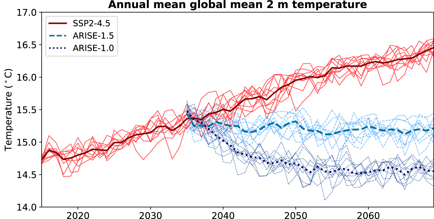
We compare the ARISE-SAI simulations with a non-SAI simulation that also uses SSP2-4.5 as its emissions scenario (hereafter SSP2-4.5). SSP2-4.5 begins in 2015 and runs through 2069. The evolution of annual mean global mean 2 m temperature for the three simulations is shown in figure 1 to demonstrate when aerosols are deployed in ARISE-SAI, and how quickly 2 m temperature diverges under all three scenarios. In SSP2-4.5, daily minimum and maximum temperature (Tmin and Tmax) were only saved for five ensemble members (006–010), so we analyse those five members in this study. Given the importance of accounting for the effects of natural variability on growing conditions, we assess outcomes in individual ensemble members of all three simulations instead of in the ensemble mean.

Figure 1. Annual mean global mean bias-adjusted 2 m temperature time series from 2015-2069 for SSP2-4.5 (red) and from 2035-2069 for ARISE-SAI-1.5 (blue) and ARISE-SAI-1.0 (purple). Thin lines are individual ensemble members; thick lines are the ensemble means.

Download figure:

Standard image High-resolution image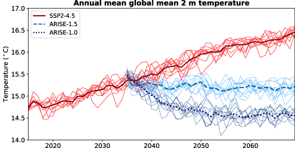

We bias-adjust the projected raw daily ARISE-SAI and SSP2-4.5 data using the quantile delta mapping method [83], and then average the adjusted daily data into monthly data when required. For the bias-adjustment, we use a three-member ensemble mean of 1980–2014 daily data from a CESM2(WACCM6) historical run as the historical model data. The historical model data is compared against daily data from ECMWF Reanalysis v5 (ERA5 [84]) to adjust projected temperature data, the Global Precipitation Climatology Project (GPCP [85]) to adjust projected precipitation rate and accumulation data, and the Atmospheric Infrared Sounder (AIRS [86]) to adjust projected relative humidity data. All data for bias-adjustment were conservatively remapped to the CESM2 grid. Due to an error, the CESM2(WACCM6) historical run did not save Tmin or Tmax. We therefore use a 10-member ensemble mean of daily Tmin and Tmax from the CESM2 Community Atmosphere Model version 6 (CAM6) historical run to adjust those fields. CESM2(CAM6) and CESM2(WACCM6) have the same model configurations except for the atmospheric component: WACCM6 has a higher upper height bound compared to CAM6 and fully resolved tropospheric and stratospheric chemistry [73, 87].

Here, we focus on three regions of interest where luxury crops currently grow: western Europe, west Africa, and northern South America. Over land in all ensemble members, temperature in all three regions was bias-adjusted by 0.5% relative to the original model output. Similarly, relative humidity was bias-adjusted by 0.5% in west Africa and northern South America, and by ∼5% in western Europe. Bias-adjusting precipitation resulted in a 24% increase in western Europe, a ∼12% decrease in west Africa, and a ∼20% increase in northern South America. Since the focus of this work is on projected changes to environmental conditions relevant for growing luxury crops, and is not meant to inform policy, we do not downscale the climate model data to avoid introducing additional uncertainties into the data.

2.2. Climate indices for crop suitability

We use several agroclimatic indices to determine macroclimate suitability for growing grapes (table 1), coffee (table 2), and cacao (table 3). Agroclimatic indices describe whether environmental variables like temperature, precipitation, and humidity exceed the criteria for suitable growing conditions. If an index is within the provided ‘unsuitable’ thresholds, growing conditions are unsuitable according to that index. For example, if a region has fewer than 50 chilling hours (table 1) during the post-harvest season in a given year, then grapes are unlikely to break their dormancy stage and growth will suffer the following year [31]. All grape and cacao indices are binary: criteria for suitable conditions are met or not. Coffee frost, maximum temperature, and Kath indices (table 2) are normalized following Dias et al [71]:

Table 1. Wine grape agroclimatic indices, affected attribute, description, threshold for unsuitable growing conditions based on the index, and time range over which the index is calculated for the Northern Hemisphere (NH) and Southern Hemisphere (SH). Tavg, Tmin, and Tmax are daily average, minimum, and maximum 2 m temperature, respectively. Pr is accumulated precipitation in mm.

CropIndex nameAttributeDescriptionThresholdMonths GrapeHuglin heliothermic [24, 88]TemperatureTemperature accumulation above 10 ∘C, adjusted for latitude1400 or 3000NH: Apr-Sep; SH: Oct-Mar Chilling hours [31]TemperatureNumber of hours required for grapevines to break dormancy post-harvest50 hoursNH: Oct-Mar; SH: Apr-Sep Frost death [23]TemperatureFreezing between bud break and floweringTmin −4 ∘C for 2 days after Tavg 10 ∘C for 10 daysNH: Mar-Jun; SH: Sep-Dec Minimum temperature [16]TemperatureLow temperature threshold for cold stress/frostTmin −18 ∘CNH: Nov-Oct; SH: May-Apr Maximum temperature [32, 89, 90]TemperatureHigh temperature threshold for photosynthetic breakdownTmax 45 ∘CNH: Nov-Oct; SH: May-Apr Heat stress [91]TemperatureHigh temperature threshold for berries post- veraisonTmin 25 ∘C and Tmax 40 ∘C for 4 days, 80–100 days after Tavg 10 ∘C for 10 daysNH: Nov-Oct; SH: May-Apr Rainfall [92, 93]PrecipitationMonthly accumulated precipitationMonthly Pr 10th percentile or 95th percentile of historical averageNH: Feb-Jul; SH: Sep-Jan Branas hydrothermal [94]DiseaseSusceptibility to mildew5100 ∘C mmNH: Apr-Sep; SH: Oct-Feb

Table 2. Coffee agroclimatic indices, affected attribute, description, threshold for unsuitable growing conditions based on the index, and time range over which the index is calculated for the Northern Hemisphere (NH) and Southern Hemisphere (SH). Tavg, Tmin, and Tmax are daily average, minimum, and maximum 2 m temperature, respectively. Pr is accumulated precipitation in mm. RH is daily mean 2 m relative humidity.

CropIndex nameAttributeDescriptionThresholdMonths CoffeeFrost [95]TemperatureLow temperature threshold for cold stressTmin 4 ∘CNH: Nov-Mar; SH: May-Sep Maximum temperature [96, 97]TemperatureHigh temperature threshold for heat stressTmax 34 ∘CNH: Mar-Feb; SH: Sep-Aug Base temperature [98, 99]TemperatureAverage growing temperatureTavg 10.5 ∘C or Tavg 32 ∘CNH: Mar-Feb; SH: Sep-Aug Water supply [100, 101]PrecipitationAnnual accumulated precipitation 1000 mm yr−1NH: Mar-Feb; SH: Sep-Aug Rust [71, 100, 102]DiseaseSusceptibility to rust18 ∘C Tavg 26 ∘C and RH 75%NH: Mar-Feb; SH: Sep-Aug Brown eye spot [71, 100, 102]DiseaseSusceptibility to brown eye spot18 ∘C Tavg 24 ∘C and RH 75%NH: Mar-Feb; SH: Sep-Aug Phoma leaf spot [71, 100, 102]DiseaseSusceptibility to phoma leaf spot16 ∘C Tavg 20 ∘C and RH 75%NH: Mar-Feb; SH: Sep-Aug Berry borer [71, 103, 104]PestSusceptibility to berry borer beetle20 ∘C Tavg 30 ∘C and RH 75%NH: Mar-Feb; SH: Sep-Aug Leaf miner [71, 103–105]PestSusceptibility to leaf miner moth20 ∘C Tavg 30 ∘C and RH 65%NH: Mar-Feb; SH: Sep-Aug Kath [106]DamageProbability of coffee bean defectsPr 750 mm and Tmin 22 ∘CNH: Oct-Dec; SH: Apr-Jun

Table 3. Cacao agroclimatic indices, affected attribute, description, threshold for unsuitable growing conditions based on the index, and time range over which the index is calculated for the Northern Hemisphere (NH) and Southern Hemisphere (SH). Tavg, Tmin, and Tmax are daily average, minimum, and maximum 2 m temperature, respectively. Pr is accumulated precipitation in mm. RH is daily mean 2 m relative humidity.

CropIndex nameAttributeDescriptionThresholdMonths CacaoMinimum temperature [22, 107]TemperatureLow temperature threshold for cold stress10 consecutive days with Tmin 10 ∘CApr-Mar Maximum temperature [22]TemperatureHigh temperature threshold for heat stressTmax 45 ∘CApr-Mar Rainfall [22]PrecipitationAnnual accumulated precipitation850 mm yr−1 or 2800 mm yr−1Apr-Mar Frosty pod rot [41]DiseaseSusceptibility to frosty pod rot20 ∘C Tavg 26 ∘C and RH 90%Apr-Mar Black pod rot [39, 40]DiseaseSusceptibility to black pod rot7-day Pr 150 mm followed by -9 ∘C 7-day Tavg 34 ∘CAug-Nov Witches’ broom [37, 38, 108, 109]DiseaseLikelihood of sporing from witches’ broom fungiPr 0 mm for 21 consecutive days followed by RH 100% 4–8 weeks laterApr-Mar

where NI**ij is the normalized index value at grid cell ij, Iij is the non-normalized index value at grid cell ij, Imin and Imax are the minimum and maximum non-normalized index values, respectively. Here a normalized value 0.9 is considered unsuitable [71].

Indices are usually calculated with daily data to capture extremes that can be obscured by monthly data. All indices use daily data except for Branas hydrothermal, grape rainfall, and Kath, which use monthly mean temperature and monthly accumulated precipitation.

Since the agroclimatic indices cover the physiological extremes for each crops, we assume that all varietals and species of grapes, coffee, and cacao respond in the same way to the environmental conditions described by the indices. Additionally, even if a disease is not currently present in a region (e.g. witches’ broom has only been identified in South America and Angola [110]), unless eradicated it could move into new regions, so it is considered a potential threat everywhere a certain crop is grown. Given the resolution of available data, some factors that influence growing conditions, such as topography and sunlight under tree canopies or on hillsides [25, 111, 112] are not fully captured in the model.

Finally, we use a composite index to determine whether a given year has suitable overall growing conditions. The composite index is a well-established method to determine whether all agroclimatic indices are met [67]. If even one index falls within the ‘unsuitable’ thresholds in a given year, the composite index is not met and crop production in that year is zero [67, 68]. For this initial study, we focus on three main regions: grapes in western Europe, coffee in northern South America, and cacao in west Africa. We focus on the first 10 full production years after SAI deployment, 2036–2045, to reduce assumptions about technological advancements or adaptation techniques that may have an even larger effect on crop production than macroclimate conditions [17]. Results for 2046–2055 and 2056–2065 are very similar and are in the Supplement.

2.3. Potential luxury crop export revenue with and without SAI

We quantify SAI’s projected effects on luxury crops by assessing the difference in potential 2036–2045 revenue between the ARISE-SAI and SSP2-4.5 simulations in 18 countries or states (regions). We chose the top grape, coffee, and cacao producing regions in 2024 [11]. Total potential revenue is based on the reported 2012–2022 average export revenue from each region [11, 113], adjusted to 2024 USD values (tables A1–A3). To keep our data sources consistent, we only included export revenue [11], which only accounts for money earned by exporting wine, coffee, and cacao outside of a country’s borders. It does not include revenue from sources such as in-country sales, jobs, or tourism.

For each region we create a crop mask from CROPGRIDS, a global dataset of production and harvest area for more than 170 crops in the year 2020 [114], which only includes grid cells where the luxury crop production area is 0. To find the potential revenue in each region, we latitude-weight and average the total number of suitable years from 2036–2045 within that region’s crop mask, then find the difference in average number of suitable growing years between the ARISE-SAI and SSP2-4.5 simulations. We then multiply that number by the average crop export value for that region (tables A1–A3). As stated above, if a year is considered ‘unsuitable’ for growing a crop based on the composite index, then we assume that no quality crops are produced that year. Thus, the revenue for that year is zero.

3.1. Historic and projected environmental conditions

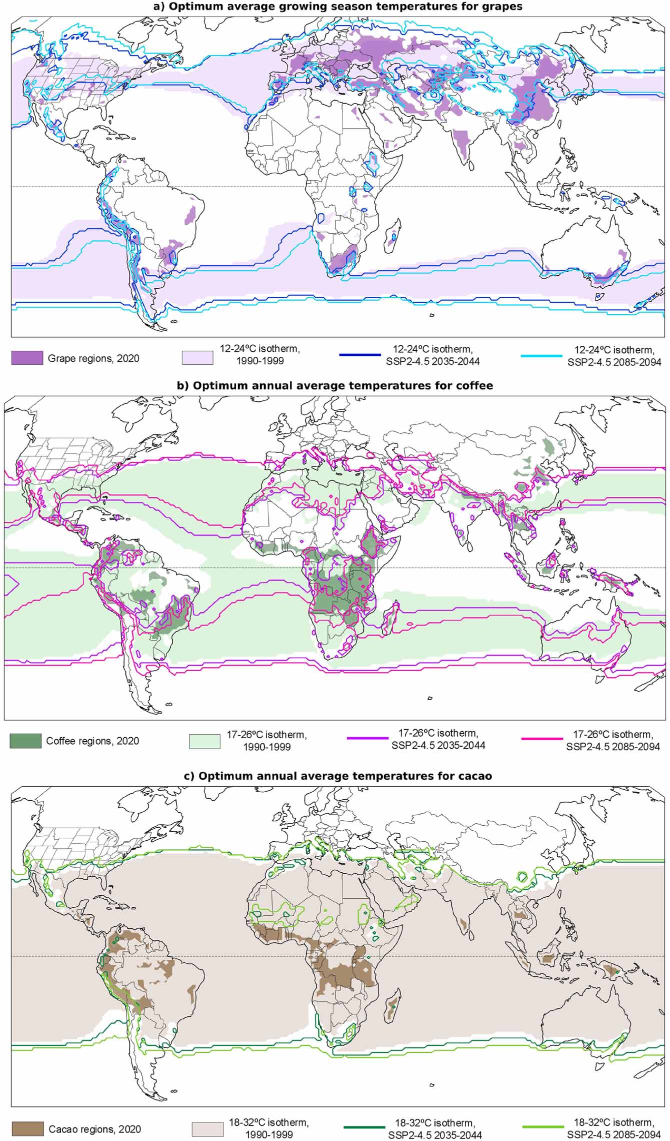
All crops have optimum temperature ranges where they grow most successfully. Since those ranges are projected to shift by the end of the century, we first show the geographic ranges of the optimum growing season and annual mean daily temperature for grapes (figure 2(a)), coffee (figure 2(b)), and cacao (figure 2(c)) from 1990–1999, and the projected geographic ranges in 2035–2044 and 2085–2094 in the SSP2-4.5 bias-adjusted ensemble mean. The darker shaded regions in each panel are where grapes, coffee, and cacao were grown in 2020 according to CROPGRIDS.

Figure 2. Historical and projected optimum daily average temperature range for (a) grapes [32], (b) coffee [21, 115, 116], and (c) cacao [16]. Lighter shading is the optimum temperature range location for each crop from 1990–1999; darker shading is where each crop was grown in 2020 [114]. Contours are the projected locations of the optimum temperature isotherms in 2035–2044 and 2085–2094 in the SSP2-4.5 10-member ensemble mean.

Download figure:

Standard image High-resolution image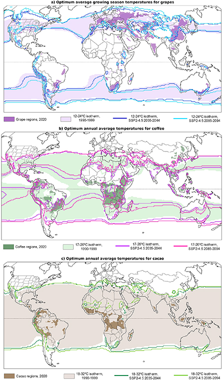

Based on temperature alone, the suitable growing area for grapes is projected to decrease by 7% by 2035–2044 and by 11% by 2085–2094 relative to the suitable growing area in 2020. Regions at the lower latitudes of where grapes are grown, such as Spain, Australia, and China, are projected to lose the most growing area. Coffee is projected to lose 29% of its growing area by 2035–2044 and 52% by 2085–2094. Much of the lost area due to temperature change alone is in Brazil, the world’s largest coffee producer. The global area suitable for growing cacao, however, is projected to increase by 3%–5% relative to 2020 suitable area by the end of the 21st century. While temperature is a major concern for the future viability of growing luxury crops, it is not the only relevant environmental condition. We next present how the composite index, a metric that assesses the combination of temperature, precipitation, and humidity, compares between the ARISE-SAI and SSP2-4.5 simulations.

3.2. Difference in number of suitable growing years with and without SAI

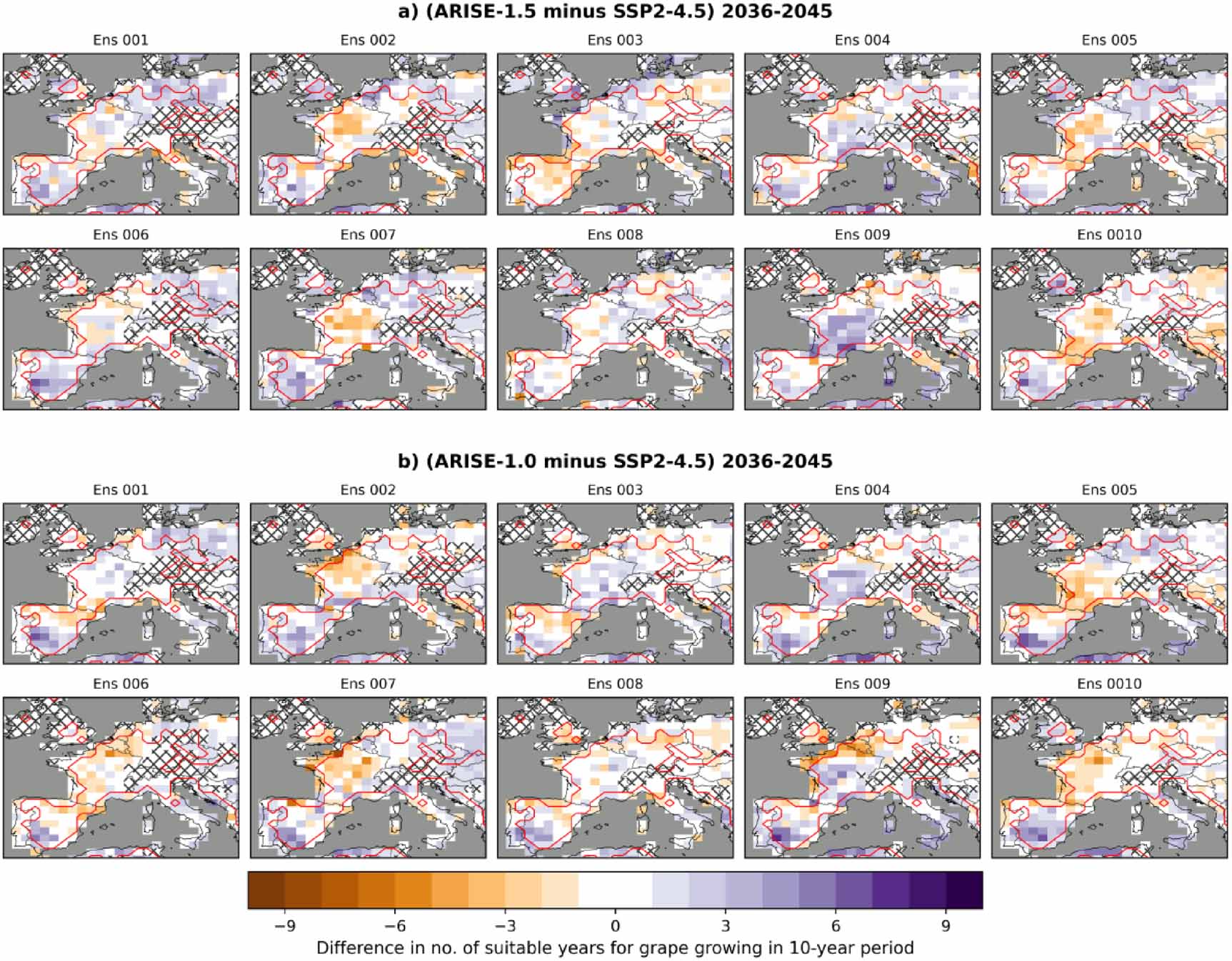
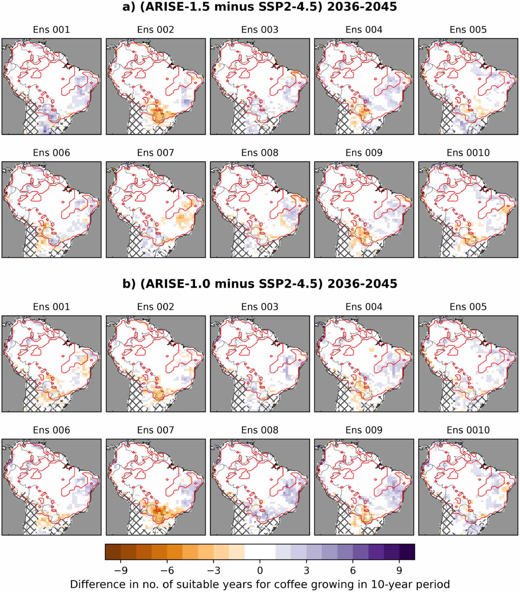
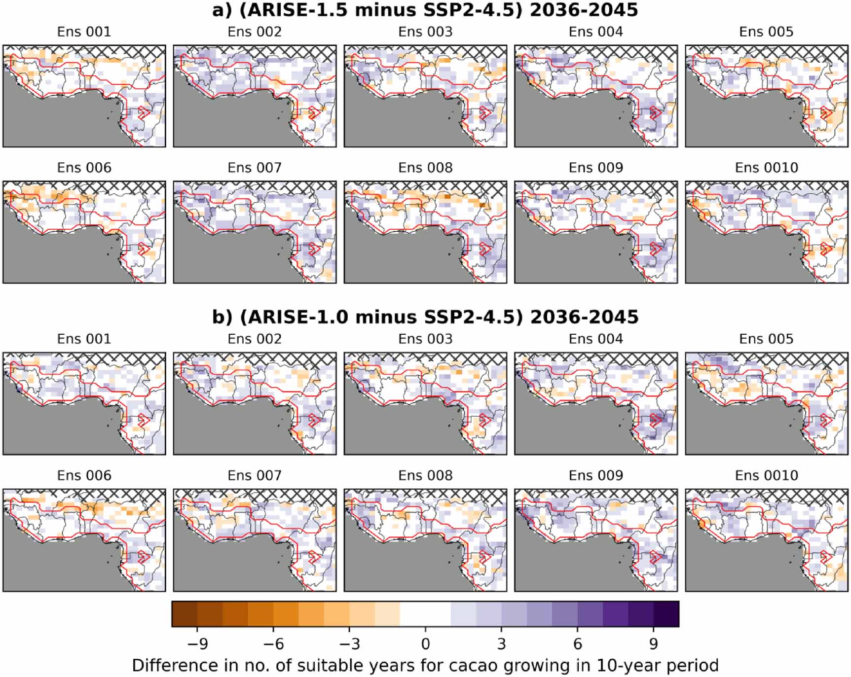
We first present the difference in number of suitable years from 2036–2045 between each ARISE-SAI ensemble member and each SSP2-4.5 ensemble member based on the composite index. Since there are only five SSP2-4.5 ensemble members, the first row in each panel in figures 3–5 is ARISE-SAI members 001–005 minus SSP2-4.5 members 006-010, and the second row is ARISE-SAI members 006-010 minus SSP2-4.5 members 006-010.

Figure 3. Difference in number of years with suitable environmental conditions for growing wine grapes in each ensemble member in (a) ARISE-1.5 minus SSP2-4.5 and (b) ARISE-1.0 minus SSP2-4.5 from 2036–2045. Purple (orange) indicates more (fewer) suitable years under SAI. Hatched regions are where there are zero suitable growing years in both the ARISE and SSP2-4.5 simulations. Red contour lines indicate grape-growing regions in 2020 [114].

Download figure:

Standard image High-resolution image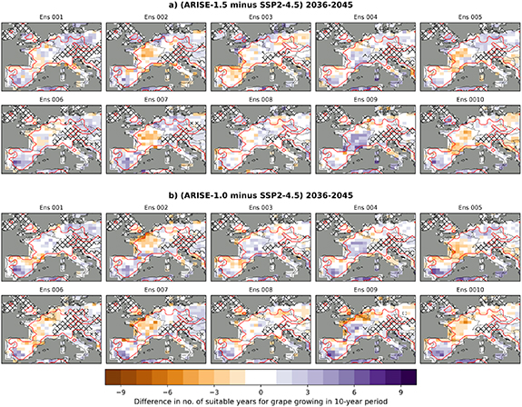

Figure 4. Difference in number of years with suitable environmental conditions for growing coffee beans in each ensemble member in (a) ARISE-1.5 minus SSP2-4.5 and (b) ARISE-1.0 minus SSP2-4.5 from 2036–2045. Purple (orange) indicates more (fewer) suitable years under SAI. Hatched regions are where there are zero suitable growing years in both the ARISE and SSP2-4.5 simulations. Red contour lines indicate coffee-growing regions in 2020 [114].

Download figure:

Standard image High-resolution image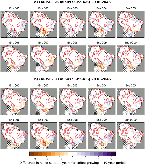

Figure 5. Difference in number of years with suitable environmental conditions for growing cacao in each ensemble member in (a) ARISE-1.5 minus SSP2-4.5 and (b) ARISE-1.0 minus SSP2-4.5 from 2036–2045. Purple (orange) indicates more (fewer) suitable years under SAI. Hatched regions are where there are zero suitable growing years in both the ARISE and SSP2-4.5 simulations. Red contour lines indicate cacao-growing regions in 2020 [114].

Download figure:

Standard image High-resolution image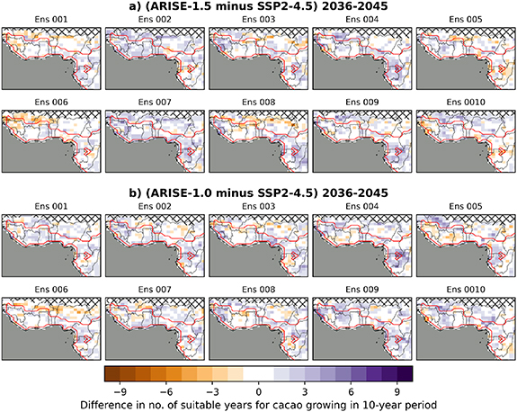

The composite index for grapes shows a wide range of responses to SAI across Europe, between ensemble members and between the two ARISE-SAI scenarios (figure 3). Hatched grid cells indicate where the difference in suitable years is zero because there are zero suitable growing years in both ARISE-SAI and SSP2-4.5. Generally, there are more suitable growing years at lower latitudes under SAI compared with SSP2-4.5. There is a robust response across ensemble members in southern Spain: in 80% of the ensemble members there are more suitable years under ARISE-1.5 and ARISE-1.0 than under SSP2-4.5 (dashed regions in figure B1). Cooler temperatures in an SAI vs a non-SAI world mean that there are more suitable years according to the Huglin index in all ARISE-SAI ensemble members compared to SSP2-4.5 (figures B2–B4). Additionally, southern Spain does not get cold enough in some SSP2-4.5 ensemble members to achieve the requisite chilling hours for grapevines to break dormancy, so suitable conditions under the chill index are only met under SAI. In later decades, Spain is still the only grape-growing region with a robust response to SAI (figures B5 and B6), even as the temperature difference between the SAI and non-SAI scenarios increases (figure 1).

Perhaps surprisingly, the likelihood of frost death is higher under SSP2-4.5 than either of the ARISE-SAI scenarios. Frost death occurs in the spring when frost kills sensitive grapevine buds. With increasing temperatures under SSP2-4.5, buds burst earlier in the spring [17], leaving them more vulnerable to mid- or late-season frosts. Stabilizing or reducing temperature under SAI reduces the incidence of mildew, which improves growing suitability based on the Branas index. In some regions, however, the Branas index cancels out the minimum temperature index: cooler temperatures increase suitability under the Branas index but can make it too cold under the minimum temperature index, leading to a negligible change in suitability based on the composite index.

The South American coffee response to SAI is also highly variable across space and ensemble member (figure 4). The largest signal is in eastern Brazil, an important coffee-growing region, but the signal is not robustly positive or negative across ensemble members in either ARISE scenario. Unlike in grape-growing regions, there is little robust agreement for shifts in coffee-growing conditions in South America under SAI (figure C1). Frost and water supply indices have the largest impact on the composite index (figures C2–C4). Internal variability causes a large spread in whether the frost index improves or reduces suitability, since it only requires a single annual frost event to substantially damage coffee crops for that year. Dry conditions also negatively impact coffee crops [100, 101]: an increase in rainfall in eastern Brazil under SAI generally leads to more suitable years based on the water supply index in both ARISE-SAI scenarios compared to SSP2-4.5 (figures C2–C4). As SAI continues, however, the coffee-growing region in eastern Brazil shifts from a positive to a robustly negative response to SAI (figures C5 and C6), particularly under ARISE-SAI-1.0.

The difference in suitable cacao growing years with and without SAI (figure 5) follows similar patterns to grapes and coffee: it is characterized by high regional and inter-ensemble member variability. The most robust signal is in Cameroon under the ARISE-1.0 scenario, where SAI leads to more suitable growing years in 80% of the ensemble members (figure D1). Accumulated precipitation has the largest influence on the composite index, which directly affects the likelihood of black pod rot disease (figures D2–D4). The maximum temperature index has no impact on cacao growing suitability in west Africa under either SAI scenario. In later decades there are more suitable years under ARISE-SAI than SSP2-4.5 (figures D5 and D6), but much of the robust signal is outside the cacao-growing regions.

3.3. Economic implications of growing crops with and without SAI

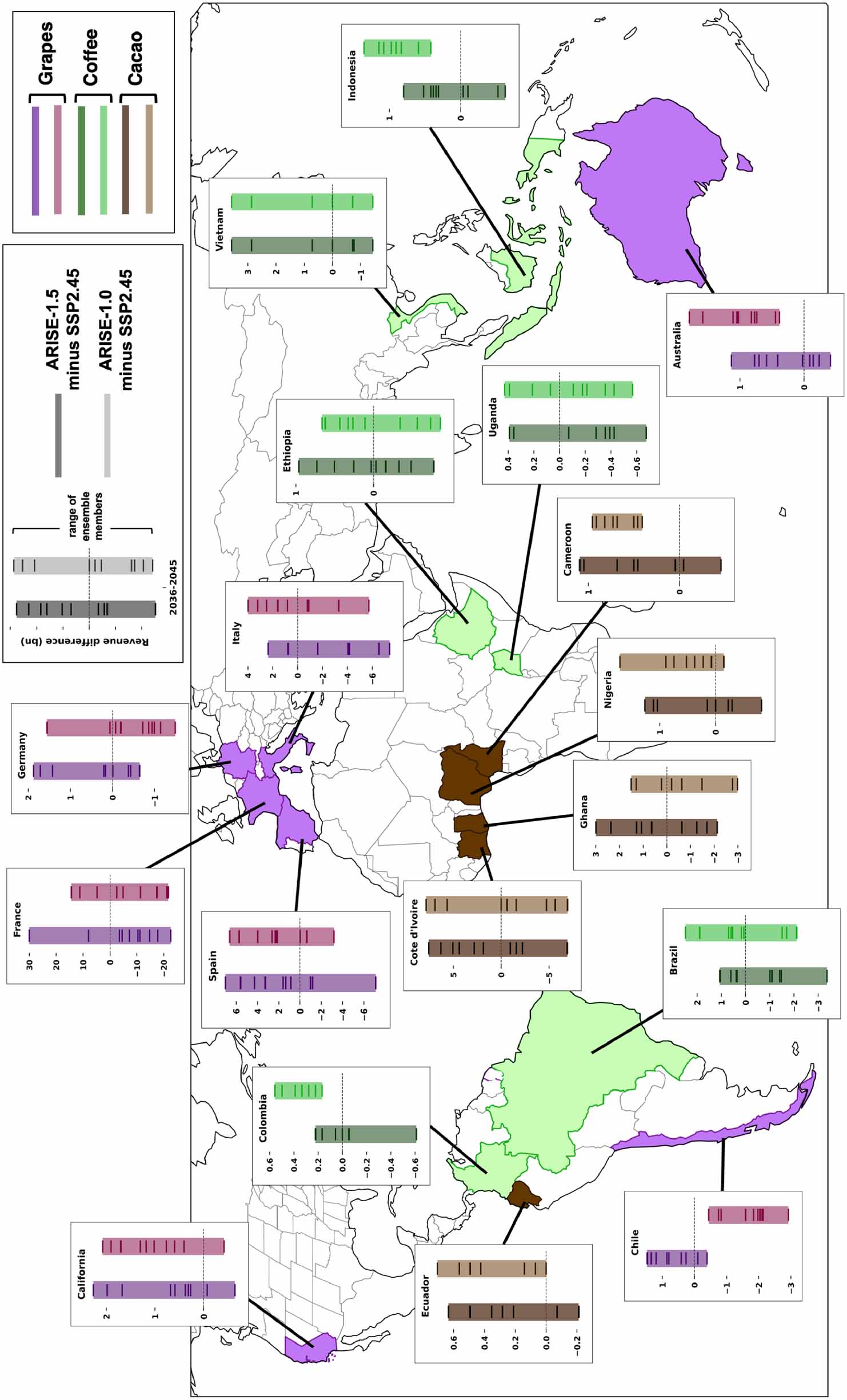
Finally, we show the potential difference in export revenue for luxury crops in 18 regions between ARISE-SAI and SSP2-4.5 (figure 6). Since we assume no quality crops are produced in a given year if the composite index is not met, the revenue differences shown here can be thought of as upper limits based on historic revenue data (tables A1–A3). The bars in each panel show the range of revenue differences for each ensemble member. In most regions, there is a large inter-ensemble member spread in revenue difference, indicating that the economic response to SAI is highly responsive to natural variability. That is, whether a region may earn more revenue from luxury crop production in a future under SAI compared to a world without SAI is highly dependent on conditions experienced under a specific climate realization. For example, there is a nearly $60 billion USD difference between the ensemble members with the highest and lowest grape revenue difference between ARISE-1.5 and SSP2-4.5 in France. In only six of the 18 regions are the differences uniformly positive or negative under an SAI scenario, and that is only true for the ARISE-1.0 scenario. Even after multiple decades of SAI deployment, revenue differences are only uniformly positive or negative in 8 of the 18 regions (figures E1 and E2). By 2056–2065, for example, revenue differences are positive under both ARISE-SAI scenarios for grapes in California, but uniformly negative for grapes in Chile and coffee in Vietnam. All regions are still projected to earn revenue from growing luxury crops in all three simulations (figures E3–E5).

Figure 6. Difference in 2036–2045 potential export revenue in billions USD for ARISE-1.5 minus SSP2-4.5 (left bar in each box) and ARISE-1.0 minus SSP2-4.5 (right bar in each box) for grapes, coffee, and cacao. Purples are grapes, greens are coffee, and browns are cacao revenue. Each horizontal line in the bars is the potential export revenue difference for a single ensemble member. Export calculations are based on average 2012–2022 revenue values in tables S1-3.

Download figure:

Standard image High-resolution image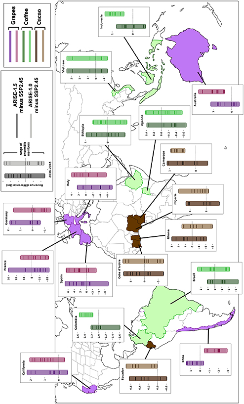

To first order, our results demonstrate that SAI may not be reliably beneficial for growing luxury crops in the future, despite reducing mean temperature and the risk of extreme heat events. This may be surprising, since heat stress is currently a major concern for grapes, coffee, and cacao. However, luxury crops are also highly sensitive to shifts in precipitation and humidity, not just to temperature. Given the large spread in outcomes between ensemble members in all three decades of SAI deployment (figures 3–6 and E1, E2), the environmental conditions suitable for growing these three luxury crops are highly sensitive to natural climate variability, and are therefore also highly dependent on the climate realization.

Part of SAI’s variable impact on luxury crops may also be due to risk tradeoffs. Reducing the risk of some adverse conditions, such as extreme heat, under SAI could be compensated for by increasing the risk of other adverse conditions, such as erratic precipitation or higher humidity. When assessing whether SAI could be beneficial or detrimental to growing luxury crops, it is also important to consider which risks are most easily managed. For example, a lack of rainfall can be, in many places, remedied by irrigation, but it is difficult to protect crops against intense rainfall or flooding. If SAI leads to fewer suitable growing years because of a manageable condition, but otherwise improves unmanageable conditions, it may be considered a more desirable strategy for addressing climate change’s impacts on luxury crops.

These results provide a framework for considering luxury crops’ heterogeneous responses to two different SAI scenarios. Given the range of outcomes across different possible future worlds, it is critical to assess responses in multiple ensemble members and not simply draw conclusions from an ensemble mean (i.e. the forced climate response). While our results should not be used to inform policy decisions around agriculture, due to the limitations of present-generation climate models and the assumptions in economic projections, they are valuable for showing the wide range of possible outcomes under SAI. Few places are likely to experience uniformly beneficial or detrimental luxury crop growing conditions after SAI deployment.

We declare no commercial or financial conflicts of interest for this research. We thank B. Dobbins for providing access to the unprocessed ARISE-SAI-1.0 output data, and C. Connolly for valuable comments on the economic perspective of this study.

All unprocessed data for the ARISE-SAI and SSP2-4.5 simulations are available from [117–119]. All Python code for the analysis is available at [120]. The data that support the findings of this study are openly available at the following URL/DOI: https://doi.org/10.5065/9kcn-9y79, https://doi.org/10.26024/0cs0-ev98, https://registry.opendata.aws/ncar-cesm2-arise/.

This research was supported by Quadrature Climate Foundation Grant 01-21-000338 and Founder’s Pledge award 240905.

Table A1. Export revenue for wine in billions USD, 2024 value [11, 113].

Year	Australia	California	Chile	Germany	France	Italy	Spain
2012	2.89	1.74	2.49	1.70	13.97	8.33	4.30
2013	2.61	1.94	2.58	1.73	14.18	9.09	4.64
2014	2.43	1.85	2.50	1.64	13.83	9.11	4.54
2015	2.37	1.97	2.47	1.41	12.37	8.07	3.99
2016	2.40	1.96	2.45	1.34	12.12	8.27	3.92
2017	2.75	1.81	2.63	1.44	13.42	8.81	4.27
2018	2.85	1.67	2.55	1.44	14.11	9.30	4.46
2019	2.67	1.54	2.40	1.35	13.65	8.91	3.87
2020	2.56	1.39	2.23	1.28	12.32	8.87	3.79
2021	1.91	1.49	2.30	1.37	15.31	9.89	4.11
2022	1.71	1.40	2.07	1.19	14.15	8.99	3.51
Average	2.47	1.71	2.43	1.44	13.59	8.88	4.13

Table A2. Export revenue for coffee in billions USD, 2024 value [11, 113].

Year	Brazil	Colombia	Ethiopia	Indonesia	Uganda	Vietnam
2012	8.22	2.73	1.01	1.82	0.56	4.51
2013	6.66	2.63	0.78	1.77	0.57	3.56
2014	8.29	3.39	0.97	1.49	0.59	4.18
2015	7.67	3.46	1.05	1.73	0.58	3.33
2016	6.65	3.25	0.92	1.40	0.50	4.17
2017	6.27	3.37	1.13	1.68	0.74	4.00
2018	5.70	2.96	0.66	1.13	0.61	3.99
2019	5.82	2.93	1.10	1.18	0.56	3.03
2020	6.19	3.10	1.09	1.06	0.66	2.77
2021	6.98	3.74	1.35	1.05	0.83	2.75
2022	9.57	4.48	1.67	1.37	0.81	3.64
Average	7.09	3.28	1.07	1.43	0.64	3.63

Table A3. Export revenue for cacao in billions USD, 2024 value [11, 113].

Year	Cameroon	Cote d’Ivoire	Ecuador	Ghana	Nigeria
2012	0.74	5.04	0.65	4.18	2.88
2013	0.77	5.75	0.74	3.32	1.22
2014	0.92	6.96	1.01	4.22	1.09
2015	1.11	7.47	1.15	4.03	0.86
2016	1.05	6.92	1.00	3.67	1.10