1748-9326/20/11/114071

Abstract

Governments worldwide are adopting ambitious policies to reduce greenhouse gas (GHG) emissions. A New York State (NYS) legislative mandate requires net zero statewide GHG emissions by 2050 in part through decarbonizing electricity generation. However, increasing renewable energy capacity, including utility scale solar (USS), competes with land-uses such as agriculture and forestry. This case study evaluates USS historic land use to project future demand for land to meet NYS’s 2050 GHG goal. Data collected from open-source solar databases were combined with USS boundaries obtained through manual and automated digitization and Monte-Carlo and Maximum Entropy modeling were used to project the likely area and land use characteristics of future sites built to meet the projected 2050 demand for electricity. Demand for solar energy in NYS is projected to reach 116–125 terawatt hours per year by 2050, when electrification of current fossil-fueled heating and transportation sectors is taken into account. By analyzing the performance of over 300 existing USS sites across NYS, we project that approximately 100 GWDC of USS capacity can meet this demand. We found an average power density of 0.62 MWDC/ha of land for fixed axis sites and 0.59 MWDC/ha for single axis tracked sites. Stochastic modeling of power density trends over time indicates that the 2050 mandate will require between 71,072 and 128,784 hectares (ha) depending on siting variables. If trends continue, we project that between 21 386 and 27 233 ha of cropland and between 14,985 and 18,463 ha of forest could be converted to USS. For future scenarios in which conversion of annual row crop land and high-quality soils were limited, there was an increase in distance to transmission lines, number of parcels required, and complexity of site shapes, which would likely increase solar development costs. These results help bound the likely land use changes that will occur to meet electric sector GHG mitigation mandates. These results also provide information about the benefits and trade-offs of restricting the conversion of current agricultural land to solar energy production. Additionally, the approach we developed, combining analysis of fenced area, capacity factors, trends in power density over time, and projecting likely future locations for solar stochastically is applicable to many global regions with solar development on agricultural lands.

Export citation and abstractBibTeXRIS

AC	Alternating current
CDL	Cropland data layer
CF	Capacity factor
CFm	Modeled capacity factor
CLCPA	New York State Climate Leadership and Community Protection Act
CNN	Convolutional neural network
DC	Direct current
DER	Distributed Energy Resources
EIA	Energy Information Administration
FA	Fixed axis
FAL	Former agricultural land
GHG	Greenhouse gas
GIS	Geographic Information System
GW	Gigawatt
GWh	Gigawatt hour
H	Hour
Ha	Hectare
IPCC	Intergovernmental Panel on Climate Change
LUC	Land use change
MSG	Mineral soil group
MW	Megawatt
MWDC	Megawatts of direct current
NAIP	National Agriculture Imagery Program
NASS	National Agricultural Statistics Service
NLCD	National Land Cover Dataset
NYS	New York State
NYSERDA	New York State Energy Research and Development Authority
NYISO	New York Independent System Operator
ORES	Office of Renewable Energy Siting
SAT	Single axis tracked
USDA	United States Department of Agriculture
USPVDB	U.S. Large Scale Photovoltaic Database
USS	Utility scale solar
YOLO	You only look once

In response to escalating risks of climate change, governments worldwide are introducing ambitious climate goals to reduce GHG emissions, decrease fossil fuel dependence, and support resilience. For example, NYS passed comprehensive climate policy (Climate Leadership and Community Protection Act, CLCPA) mandating zero GHG emission electricity generation by 2040 (Senate Bill S6599 2019). This goal includes increasing the use of renewable energy, including USS, herein defined as a ground mounted solar site with a DC capacity greater than one megawatt (MWDC). The land requirements to meet these solar goals are substantial, causing concern about competition between USS and agricultural production (Nonhebel 2005, Cunningham and Seidman 2024). NYS estimates it will need to produce 95 400 GWh with USS (NYSCAC 2022).

The dominant method of USS land acquisition is through long-term leases, sometimes valued at $1000 acre−1 yr−1 for the landowner, or approximately ten times the rental rates for commercial agriculture (solarlandlease.com 2020, Inc n.d.). Important land characteristics desirable for agriculture are also desirable for solar, including flat or low slope, road access, and proximity to power lines (Katkar et al 2021). Competition for land between agriculture and solar is increasing land rental rates of farms in areas suitable for solar development, and may have far reaching impacts on the success of agricultural communities (Li et al 2024). In 2023, NYSERDA crafted policies to incentivize solar on less productive agricultural land or allowing dual-use systems (requiring some form of agricultural co-production on USS sites) (RESRFP23-1 Appendix 2 2023). Quantifying these land conflicts is beginning to be addressed in the literature, but the regional and temporal variation in solar power output, and fragmented nature of renewable energy targets make these analyses difficult to extrapolate from, both geographically, and into the future (Horner and Clark 2013).

There is a large body of emerging research analyzing trends in solar land use through remote sensing (Bolinger and Bolinger 2022, Blaydes et al 2025, Goosay n.d.), Previous research has extrapolated solar area from known relationships (Katkar et al 2021). More recent research has taken solar land use analysis a step further and predicted future land conversion to solar based on legislative goals for future renewable generation (Van De Ven et al 2021, Blaydes et al 2025). However, to the authors knowledge, no research exists that attempts to harmonize existing land use trends and policy goals to define not just how much land will be converted to solar, but what types of land and the quantity of each. In this paper, the authors attempt to fill that gap by estimating land conversion impacts due to existing solar sites, as well as predicted future sites using new methods and modeling. While not intended to be a one to one prediction of future solar development, our results illustrate how NYS agricultural land could be impacted if current trends in USS siting continue into the future under a scenario where climate goals are met.

Methods, including the key data sets, analytical steps, and results are summarized in figure 1.

Figure 1. Methodology flow chart. Abbreviations: CDL: cropland data layer, CLCPA: Climate Leadership and Community Protection Act, MSG: mineral soils group, USPVDB: United State Photovoltaic Database, NAIP: National Aerial Imagery Program, MaxEnt: maximum entropy.

Download figure:

Standard image High-resolution image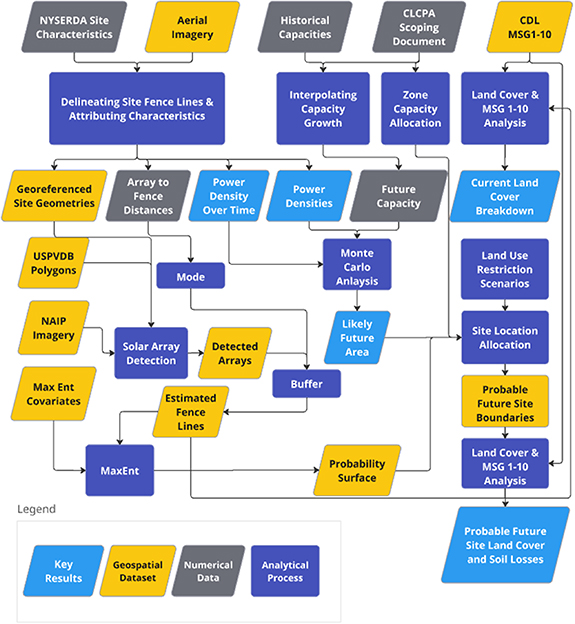

2.1. Site power density and trends over time

We divide NYS USS systems into three groups, (1) Single Axis Tracked (SAT), (2) Fixed Axis (FA), and (3) large sites (LGs). SAT sites have a tracking mechanism to angle the panels to follow the sun throughout the day, while fixed axis sites do not. LGs are over 25 MW in capacity, and fall under a different regulatory structure, and are therefore treated as their own category. We assumed that LG sites consist of mainly SAT arrays based on publicly available project applications, but since no such sites had been completed in NYS at the time of the analysis, this assumption cannot be confirmed. Rather than assume a specific mix of SAT, FA and LG sites in the future, we analyzed each site type separately, assuming it would meet the entire energy demands of the state, so that any mix of site types can be evaluated based on our results.

Site characteristic data were obtained from the NYSERDA DER, which compiles site performance and location data for USS that receive state funding (Open NY Data 2024). Site type (SAT or FA) is not explicitly stated in the DER dataset, however, each site includes an estimated annual energy production value in kWh yr−1, which is calculated using a different CF for each site type. This estimated energy production value allowed site type to be determined by back-calculating the site modeled capacity factor (CFm) used to estimate yearly output (CFm, equation (1)). The NYSERDA DER database uses CFm values of 15.99 for all SAT and 13.39 for all FA sites. Once site type was assigned to each dataset by CFm, (Sites with CFm of 13.39 were assumed to be FA, while sites with CFm of 15.99 were designated as SAT), the value was not used in any further analysis.

For small USS sites (greater than 1 MW and less than 25 MW), a randomized subset of 200 SAT and 200 FA sites was extracted from ∼1200 sites listed in the DER dataset and each site was viewed with the orthoimagery provided as a webservice layer in ArcGIS Pro. Of 400 selected sites, 108 FA sites and 85 SAT sites were covered by orthoimagery with adequate resolution to delineate fences as shown in figure 2. Capacity (C) and project application dates were attributed to the fence line polygons from the DER dataset. Power density (MWDC/ha) was calculated by dividing site capacity by the calculated area of the fence polygons.

Figure 2. Example of manually digitized and machine-learning (YOLO) detection of a solar site. (Basemap imagery provided by ESRI ArcGIS and New York State).

Download figure:

Standard image High-resolution image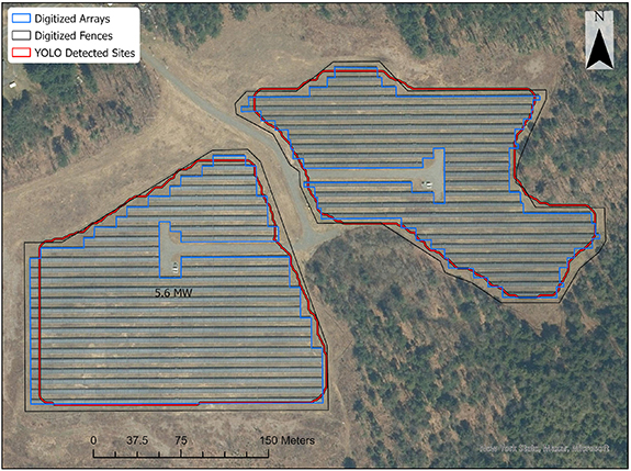

Equation 1. Modeled CF

where:

CFm = Modeled capacity factor

EP = Expected energy production (MWh yr−1)

C = Site capacity (MWDC)

8766 = Hours per year

The method for the small sites described above was applied to 11 proposed LG sites which had applications submitted to the NYS Office or Renewable Energy Siting (ORES). Since these proposed sites had not yet been installed as of the time of the analysis, fenced area was determined by digitizing site plans after they were spatially referenced. Mean and standard error of power density were calculated using the same methods as the small sites, though trends over time were not analyzed due to the limited sample size and lack of installation dates.

2.2. Capacity factor (CF)

USS site performance data, including site CFs averaged to monthly intervals, is tracked by NYSERDA and can be viewed on the DER website (NYSERDA DER Integrated Data System n.d.). Site CF values were collected by using an automation script capable of copying and pasting information from all projects listed on the DER site. Once collected, the CF values were clipped to the nearest full year (sites with less than one full year of data were excluded), and CFs were averaged for each site. To obtain individual site locations, the DER data were merged with tabular data from the OpenNY dataset by site name and address, with the resulting dataset containing 290 FA and 50 SAT sites with CF data.

2.3. Solar site detection with machine learning

To detect solar sites from remotely sensed imagery, we developed a machine learning model trained on the 2022 NAIP aerial imagery dataset as well as manually delineated solar site footprints (figure 2). Specifically, we trained a CNN using the YOLO v8 model for object detection and segmentation. The YOLO model was chosen due to its fast processing speed and skill at object detection for visually distinct but spectrally varied targets (Zhao et al 2019, Diwan et al 2023). Training data included manually delineated solar site polygons from the USPVDB as well as the small FA and SAT sites described above. The model was trained over 500 epochs, reserving 20% of the data for validation. Hyperparameters included an image chip size of 640 pixels, a patience of 20, and a dynamically configured batch size, while the learning rate remained at the default value. Commonly misidentified landscape features like silage/haylage rows, train depots, parking lots, and orchards were classified separately to enhance feature discrimination.

2.4. Existing site land use characteristics

Former land use of detected solar polygons was identified by overlay with an aggregated version of the 2008 CDL and tabulating the total area of each land class (USDA 2023).

2.5. Inverter clipping

Most USS solar sites undersize inverter capacity as sites rarely perform at peak output. Inverter clipping is the loss of solar power when the DC capacity of a solar array outperforms the AC capacity of the inverter, which converts DC to AC. The ratio of DC array capacity to AC inverter capacity is hereafter referred to as the DC:AC ratio.

To assess the potential energy production loss from different DC:AC ratios, hourly energy production data were extracted from the NYSERDA DER website using a script similar to the one used for CF data. Sites with fewer than three years of continuous recordings were excluded. Since mean hourly panel output and DC panel capacity data were available, it was possible to simulate AC output capacity values to calculate how much electricity in kWh would be lost over an average year at different DC:AC ratios. This was done by examining the DC output of the array, and capping AC output at ratios of DC capacity. For example, if a site had a DC: AC ratio of 1.5:1, with a DC capacity of 1 MW and an AC capacity of 0.75 MW, any power generated over 0.75 MW would be wasted. Simulated AC capacity limits were imposed on the data in 1% increments to simulate DC:AC ratios from 1:1 (DC panel capacity matches AC inverter capacity) to 2:1 (panel capacity is double inverter capacity). For each increment, generated electricity in excess of the imposed inverter limit was tallied to produce a total energy loss for all sites (example shown in figure S1 of the supplement).

2.6. Projecting future capacity

The NYS climate scoping plan (NYSCAC 2022) includes four scenarios to meet climate goals. In scenario 4, energy generation required from solar was projected to be 125,980 GWh yr−1 in 2050, of which approximately 95,400 GWh is from USS. We estimated the required DC USS capacity for SAT and FA sites by extrapolating from CF values obtained for each site type as well as losses due to an assumed 95% inverter efficiency and inverter clipping at an DC:AC ratio of 1:1.5 (equation (2)).

Equation 2. Capacity needed to meet 2050 solar energy goals.

where:

C = Needed capacity (GWDC)

E = Future energy goal (GWh)

CF = Capacity factor

8766 = Hours per year

CL = Clipping losses

Iη = Inverter efficiency

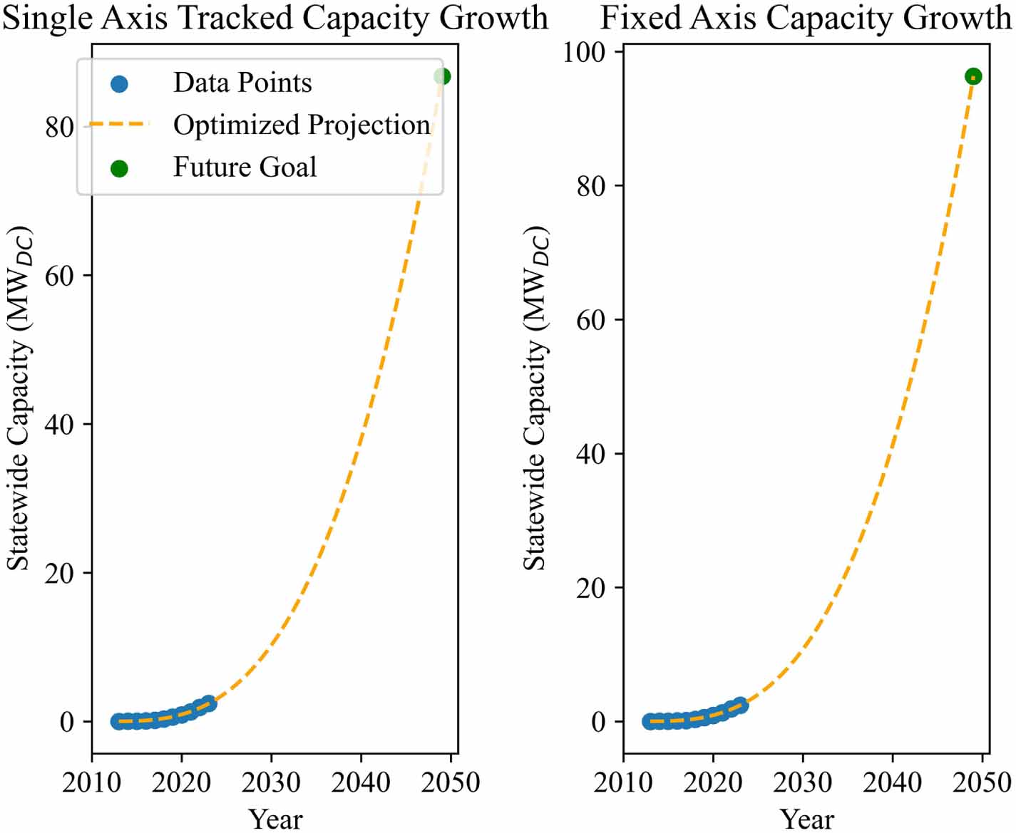
We modeled the growth rate of statewide solar capacity by summing yearly statewide capacities of USS sites by completion year, plotted against the total capacity by year, and fit a power function (equation (3)). To extrapolate growth trends to 2050, an optimization algorithm was used to iteratively adjust the power function constants to both minimize error in the historical values and the targeted capacity values for SAT and FA sites in 2050.

Equation 3. Solar PV capacity for any year since 2013

where:

Capacityyr = Total statewide USS capacity in MW at a given year

a = Constant 1

b = Constant 2

t = Year

2.7. Monte-Carlo analysis of projected future solar land area

We estimated the land area needed to reach the capacity demand for each site type by 2050 using Monte Carlo analysis. Gaussian probability density functions were defined for (1) current power density (equation (4)) and (2) the rate of power density improvement over time (equation (5)). The analysis was performed separately for FA, SAT, and LG sites. For LG sites, the same technique was used, however, we used the power density slope function from SAT sites, since there was no chronological data for the LG sites. The starting power density and the slope of the power density function varied in each Monte Carlo iteration. Limits were set to discard improbable values such as power densities greater than 2 MW DC/ha, (approximately double the highest value in our existing dataset) or power density improvement slopes that were less than zero. The analysis ran 10,000 iterations for each site type.

Equation 4. Power density for each Monte Carlo iteration

where:

PDx = Power density in the year x

y0 = Starting power density (mean PD based on 2022 imagery data)

εy0 = Random variation sampled from a normal distribution of the standard error of the mean

= Slope of power density increase per year

= Random variation in the slope, sampled from the standard error of the regression slope

= Number of years since 2000

Equation 5. Monte Carlo area extrapolation

where:

Total Area = Sum of all fenced area of solar sites in 2050 to meet net zero grid mandate

Cannual = Added total statewide capacity for a given year (MW)

PDi = Initial Power Density in 2022 (MW ha−1 of fenced area).

m = Slope of power density improvement over time (MW ha−1 yr−1).

2.8. Projecting potential future sites

To project potential future solar site locations, we developed a model to represent the likelihood of solar development on any geographical location in the state by analyzing patterns of solar site development to date. Specifically, we used a maximum entropy (MaxEnt) model because it is effective with presence-only data (Tao et al 2025). The model used existing site locations as training data along with geospatial datasets expected to influence solar site placement, such as land cover, proximity to infrastructure, and topography as covariates (table 1). The model generated a probability surface indicating likelihood of future solar site development for any location based on existing site characteristics.

Table 1. Covariates used in maximum entropy model to project future solar sites.

Covariate	Units	Source
Land use	Categorical	(USDA 2021)
Parcel density	Unitless	(NYS 2023b)
Distance from road	Meters	(NYS 2023a)
Slope	%	(LandFire.Gov 2016)
Land value	$/Acre	(NYS 2023b)
Soil classes	Categorical	(SSURGO n.d.)
Distance to transmission lines	Meters	(U.S. Federal Datasets 2024)

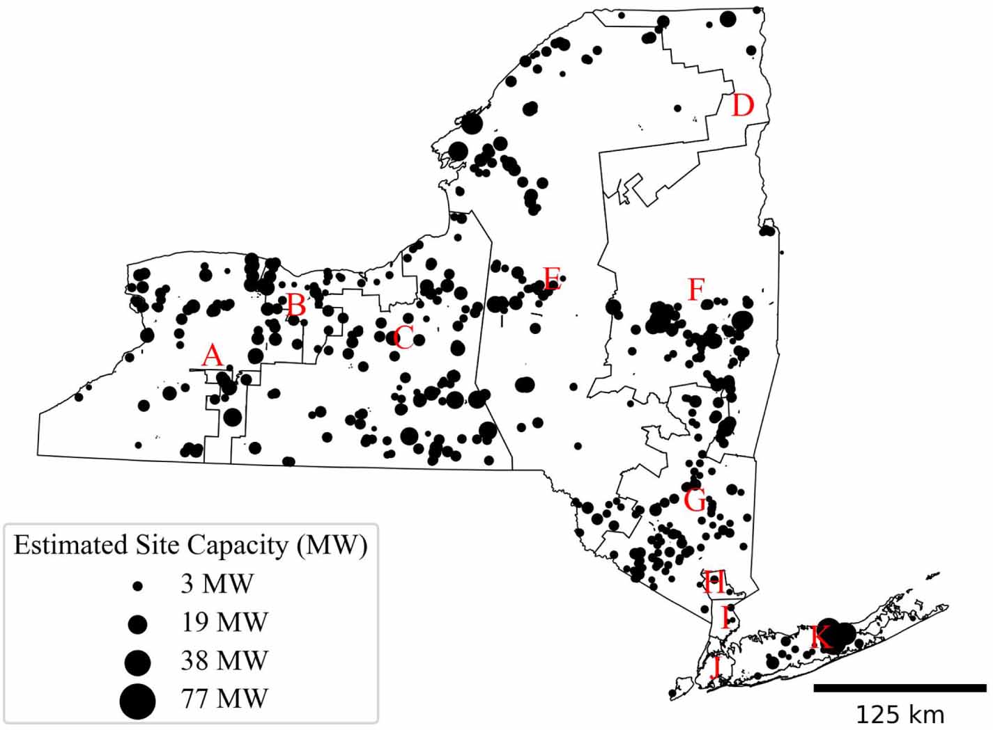
Probable solar site locations were predicted for LG, FA, and SAT sites across NYS. Sites were distributed proportionally to the NYISO load zone capacity allocations, with zone limits based on the proportion of interconnection capacity available. Zonal capacity values as a proportion of total capacity as of 2022 were: A-E: 59%, F: 32%, GHI: 6.8%, J: 0%, K: 3%, and were assumed to remain constant through 2050 (NYSCAC 2022).

An algorithm was developed to delineate site boundaries with an appropriate cumulative area for each zone, selecting sites with the highest probability scores. The algorithm accounted for improvements in site power density over time and differences in initial power density among SAT, FA, and LG sites.

2.9. Likely future site characteristics under different land use restriction scenarios

Agricultural lands were identified and classified using the CDL (USDA 2023). Soil quality was classified using MSGs, a NYS ranking system from 1 to 10, where groups 1–4 are considered high quality agricultural soils. Land classified as low-high intensity developed in the CDL was excluded from all scenarios but undeveloped land inside cities was not, allowing sites to be placed on city parks and other open spaces inside city limits, but not suburban or urban areas populated by buildings.

Polygons representing solar site allocation to only the most probable locations that do not violate scenario restrictions were generated for the following siting restrictions:

1.

No restrictions (other than developed lands).

2.

No high-quality agricultural soils (MSG 1–4) could be used.

3.

No lands currently (2023) used in row crop production (with any MSG) or high-quality soils (MSG 1–4) could be used.

Once the most probable site locations were allocated under each land use restriction scenario to reach the solar power generation target, average site characteristics including land cover, ratio of site area to perimeter, distance to the nearest transmission line, and average parcel size were calculated.

2.10. Future crop area loss

To project crop area losses due to future solar development, under different siting restrictions scenarios, site boundaries were predicted to simulate site placement when no restrictions (scenario 1), no high-quality agricultural soils (scenario 2) and no agricultural or high-quality soils (scenario 3) were available to the placement algorithm. The resultant polygons were overlaid on an aggregated classification of the CDL containing the following categories: not Crop, Corn, Soybean, Alfalfa, Hay, Wheat, Oats, Beans, Barley, Other, Grass, Rye. All cells with centroids within a projected future site polygon were summed into crop totals and the area of cropland occupied was divided by state total harvested land for each crop.

2.11. Accounting for FAL

To account for misclassification of abandoned agricultural land as active in the CDL, proportions of FAL to active agricultural land were taken from Richardson et al 2023b for each land cover category (table 2). The resulting ratios were applied to the total areas of land cover we identified as currently occupied by solar or likely to be by our MaxEnt modeling.

Table 2. Former agricultural land proportions (Richardson et al. 2023b). Note that units were converted from acres to hectares.

Land cover type	Area (ha.)	Area in agricultural production (%)	Former agricultural area (%)
Row crops/grains	711840	99	1
Alfalfa hay	265116	97	3
Other hay	541936	89	11
Fallow/idle	69060	99	1
Orchard	28818	90	10
Christmas trees	546	97	3
Pasture	618270	63	37
Non-agriculturea	410135	11	89
Persistent grassb	38670	1	0/99
Transitional forestc	53131		0/100

aNon-agriculture—Areas identified as agriculture by NLCD but that appear more similar to the other non-agricultural non-grassland categories according to CDL (shrub, forest, wetland, barren, developed, or water). Together with the two NLCD grassland types, these land cover types represent the more naturalized early successional end of the herbaceous vegetation spectrum found within agricultural settings. bPersistent grass—Persistent grasslands, excluding post-forest-disturbance areas (NLCD 71). cTransitional forest—Transitional post-timber-harvest grassland (NLCD 46) Grassland areas not included in estimate of suitable and available post-agricultural lands in New York (1.67 million acres).

2.12. Energy density

While DC capacity is commonly used in NYS legislation to set future renewable energy targets, energy production (MWh ha−1 yr−1) is more relevant for energy sources like solar PV, which have highly variable CFs and rarely reach peak output. Site CFs obtained from the methods described in the CF section above, were matched to their respective SAT or FA site types, and both present and future energy density values were calculated using equation (6), with future energy density incorporating projected area values and future capacities.

Equation 6. Energy density

where:

C = Current capacity (MW)

8766 = Hours per year (h)

CF = Empirical capacity factor (fraction)

A = Site fenced area (ha)

Future energy density for the year 2050 was calculated by dividing the most likely area value (mode) of the 2050 Monte-Carlo analysis for each site type by the statewide capacity target in MWDC used for future scenarios.

3.1. Solar site size and power density trends

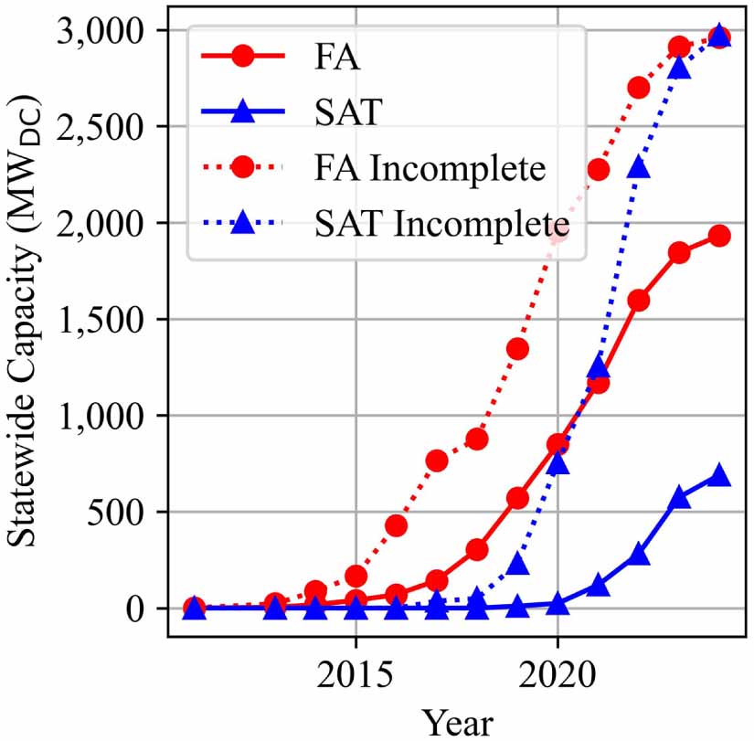
As of July 2024, there were 1243 solar sites over 1 MW in the NYSUN dataset, 515 were assumed to be SAT based on the modeled capacity factors contained within their data, while the remaining sites were assumed to be FA. Although completed FA sites outnumber SAT overall, since 2018, applications for SAT sites outnumbered those of FA sites (figure 3). Total NYS capacity for completed sites is 2419 MWDC.

Figure 3. New York Statewide utility scale solar capacity by year for fixed axis (FA) and single axis tracked (SAT) sites. Dotted lines indicate capacity based on site application year, solid lines indicate capacity based on completed sites.

Download figure:

Standard image High-resolution image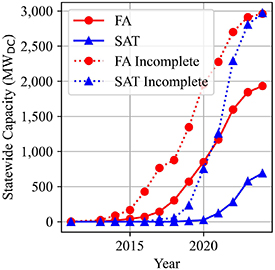

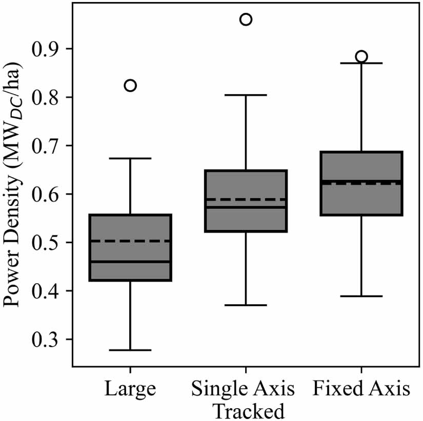
Power density was calculated as MWDC site capacity per fenced area. The power density within and among site types was variable (figure 4). Average power density was significantly higher for FA than SAT sites (t = −2.157, p = 0.032). Significance was not tested for LG sites due to low sample number. The overall average power density for all site types was 0.61 MWDC/ha.

Figure 4. Power density (MWDC/ha) of each USS type. Large site mean power density was 0.50 MWDC/ha (n = 11), single axis tracked sites mean power density was 0.59 MWDC/ha (n = 85) and fixed axis sites mean power density was 0.62 MWDC/ha (n = 108). Solid black lines represent the median, dotted lines represent the mean, and circles represent outliers.

Download figure:

Standard image High-resolution image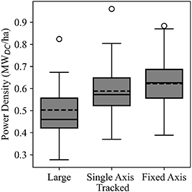

Power density increased significantly over time for both SAT and FA sites with slopes of 0.02044589 and 0.01528890 MW ha−1 yr−1 respectively (figure 5).

Figure 5. Power densities of single axis tracked (SAT) (blue triangles) and fixed axis (FA) (red circles) sites over time. The single axis power density slope is 0.02044589 and the intercept is −40.70. The fixed axis power density slope is 0.01528890 and the intercept is −30.21. SAT and FA power density trend R2 values are.049 and.062 respectively.

Download figure:

Standard image High-resolution image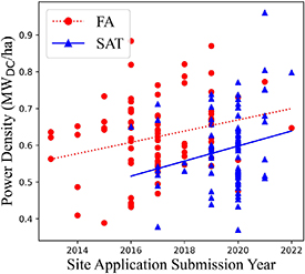

3.2. Solar site detection and segmentation with machine vision

The machine learning solar site detection model achieved reasonable rates of precision and recall with almost 2000 individual solar arrays ultimately detected and manually confirmed. After individual polygons representing detected arrays were grouped by proximity into likely sites and filtered by area, 509 sites with estimated capacities over 1 MW remained (figure 6).

Figure 6. Detected locations of 2022 solar sites within New York Independent System Operator (NYISO) load area control zones. Capacity is estimated from site size based on 1.61 ha MW−1 power density.

Download figure:

Standard image High-resolution image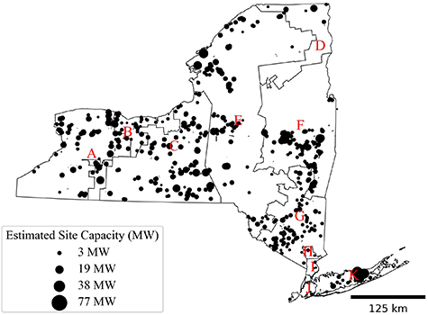

3.3. Land use and land cover change due to solar sites

The total area used by detected solar sites was 3652 ha, while the predicted area installed by 2022, based on our power density measurements and the installed capacity value from the sum of all NYSERDA DER projects was 4300 ha.

We evaluated previous land cover of detected solar sites (figure 7). Field crops (864 ha) and hay (827 ha) account for 39% of the area taken by current solar. Other land cover types converted to solar were pasture, forest, and alfalfa. Of that land area (3652 ha) 607 ha (14% of total land occupied by solar sites) could be FAL (land that was no longer in active agriculture, based on proportions from Richardson et al 2023b).

Figure 7. Prior land use area within detected solar sites. Former agricultural land (FAL) shown in the black bar is based on a separate analysis and overlaps with other categories. Land quantities are provided in table S2 of the supplement.

Download figure:

Standard image High-resolution image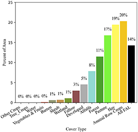

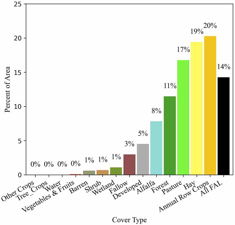
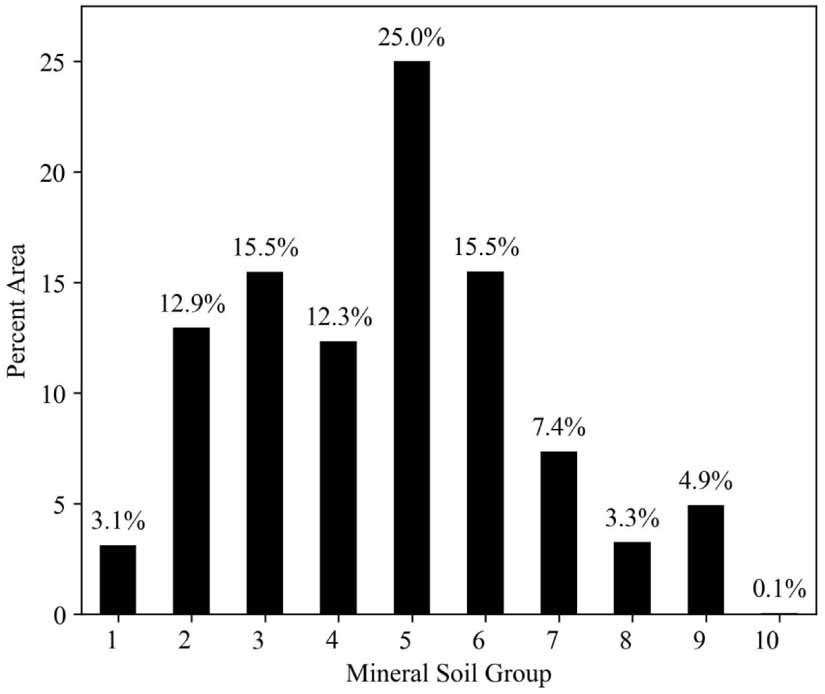
We evaluated soil quality of detected solar sites (figure 8). Solar sites most commonly occupy MSG 5 (919 ha), followed by MSG 6 (570 ha) and MSG 3 (454 ha). The area of the higher quality soils (groups 1–4), sum to 1614 ha which is 44% of the total 3677 ha.

Figure 8. Land use of existing solar sites by mineral soil groups (percentage of total area). Land area values are provided in table S4 of the supplement.

Download figure:

Standard image High-resolution image

We evaluated displaced commodity crops by detected solar sites (table 3). Of land now occupied by solar sites 72% grew commodity crops before conversion to solar.

Table 3. Area of NYS commodity crops displaced by solar sites based on 2008 cropland data layer (USDA 2023).

Crop	Total land (Ha)	Land used (Ha)	Percentage
Hay	266481	589	0.22%
Oats	18593	42	0.23%
Soy	138204	103	0.07%
Wheat	42893	207	0.48%
Alfalfa	134503	244	0.18%
Barley	2623	4	0.14%
Corn	501634	1,326	0.26%
Rye	6236	19	0.30%
Other crops	1897513	190	0.01%

3.4. Projected future capacity

Total USS capacity in the NYSUN database increased exponentially over time with equation (7) explaining 99% of the variation in capacity growth between 2013 and 2023.

Equation 7. Trend of SAT USS capacity in NYS over time

where:

Ct = Capacity at year t

t = year

Future increases in capacity were calculated by adding the 2050 capacity goal of 86 779 MWDC for SAT sites with 96 330 MWDC for FA sites from the NYS scoping plan. Current trends were fitted with exponential functions to meet 2050 anticipated demand (figure 9).

Figure 9. Projection of future solar capacity growth in New York State.

Download figure:

Standard image High-resolution image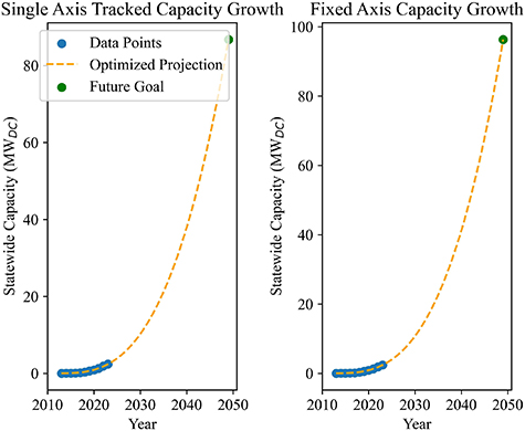

3.5. Future area projected to be occupied by USS

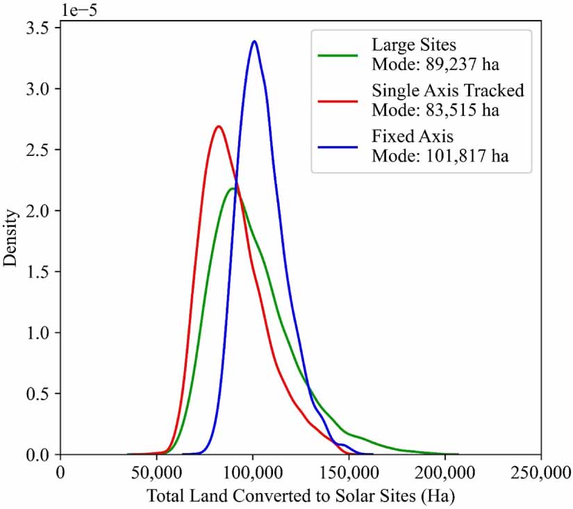
We project that total USS land area by 2050 has an 80% likelihood to be between 71072 ha and 128784 ha, depending on the mixture of site types and the future rate of increase in power density. Overall, SAT sites had the greatest probability of using the least amount of land to reach the required capacity, with a mode of 81435 ha, while FA sites had the highest probability of using the most land, with a most likely area value of 98726 ha (figure 10). These results indicate that if trends in power density continue, the aggregate power density of sites in 2050, before losses due to AC conversion, would likely be 1.07 MWDC/ha (fenced) for SAT and 0.98 MWDC/ha for FA sites.

Figure 10. Projected future New York State area required for different types of solar sites. The Y axis indicates relative probability density of each area result.

Download figure:

Standard image High-resolution image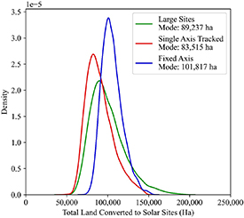

3.6. Potential future site locations

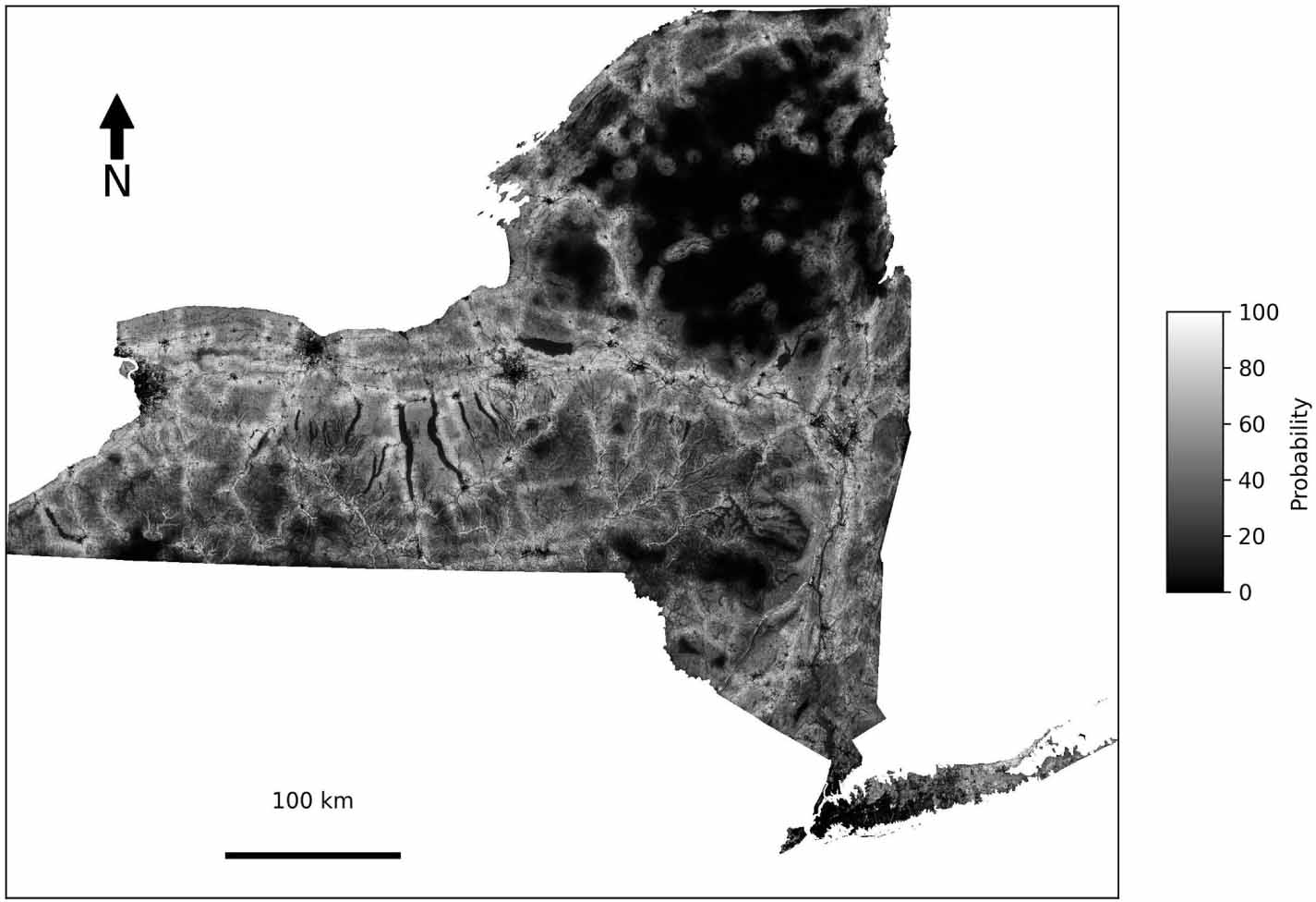
The MaxEnt model projected a probability distribution of likely solar development across all available locations in NYS at 30 m resolution (figure 11). These results are based on statistical relationships between existing sites and the spatial covariates (table 4). Based on the existing site development covariates, the majority of the available land was of low probability, with values lower than 50%. We found approximately 66000 ha of land with a probability of 90% or greater (figure 11).

Figure 11. Probability of future solar site development from the maximum entropy model.

Download figure:

Standard image High-resolution image

Table 4. Importance of covariates used to project the likelihood of future solar development by the maximum entropy model.

Variable	Percent contribution	Permutation importance	Data source
Former land use	31.2	25.7	(USDA 2023)
Parcel density	22.3	27.9	(NYS 2023b)
Distance to transmission lines	20.1	19.3	(NYS 2023a)
Soil classes (MSG 1–10)	12.9	3.1	(SSURGO n.d.)
Distance to nearest road	8.8	16.0	(NYS 2023a)
Slope	2.5	6.6	(LandFire.Gov 2016)
Assessed land value	2.2	1.4	(NYS 2023b)

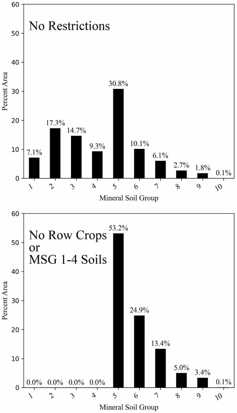
The future scenario without any land cover type or soil restrictions (scenario 1), showed solar sites displacing primarily field crops, pasture, and forest, with lesser displacement of grass hay, alfalfa and developed land (figure 12). Future scenario 2 showed a similar land use breakdown to the unrestricted scenario, but with somewhat less row crop and somewhat more hay and pasture land (figure 12). The future scenario that excluded all row cropped land and high-quality soils (scenario 3) showed the largest difference in LUC, with solar sites replacing substantial amounts of pasture land (figure 12). Detailed breakdowns of each crop-scenario combination are in table S1 of the supplement.

Figure 12. Effect of each future scenario on the displacement of prior land uses for single axis tracked solar site development. Former agricultural land (FAL) shown in the black bar is based on a separate analysis and overlaps with other categories. Area values show in table S1.

Download figure:

Standard image High-resolution image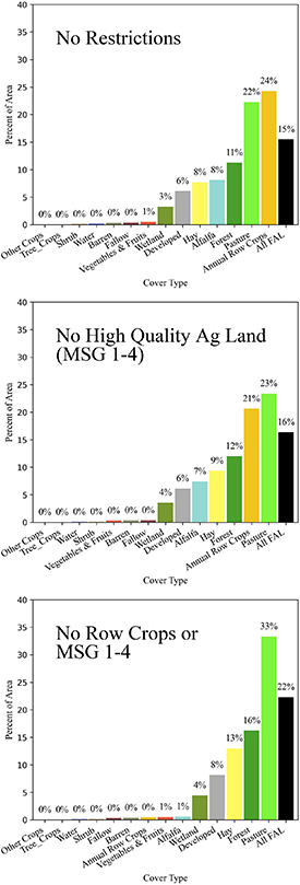

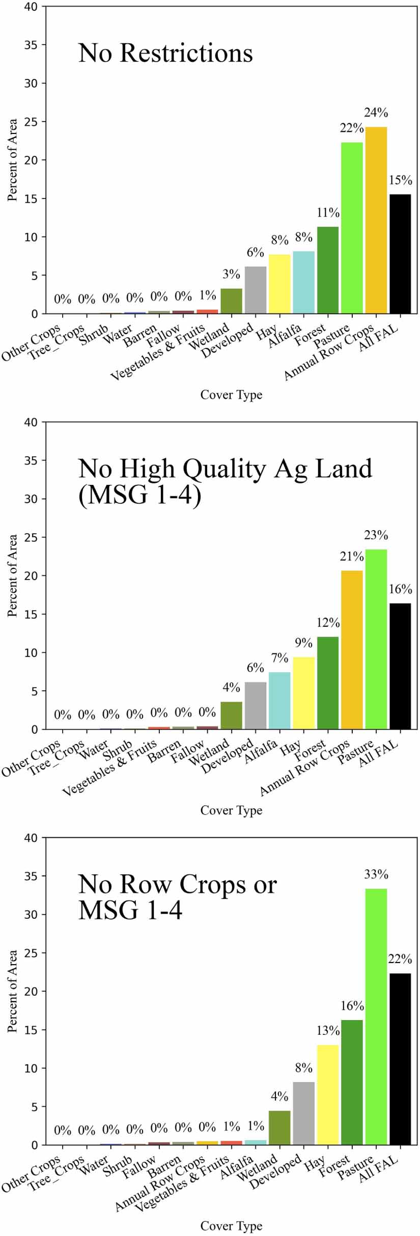
The future scenarios also used soils of different quality for agricultural production (figure 11). The scenario with no restrictions showed solar sites displacing primarily MSG 5, 2, 3, and 6, with 50% in MSG 1–4. Both scenarios that restricted future site allocation on MSG 1–4 showed the majority of sites placed on MSG 5, with additional groups having decreasing area from groups 6–10 (figure 13). The effects of potential future sites under different site types and land use scenarios on commodity crops based on 2023 crop data are in table S4 and figure S1 of the supplement.

Figure 13. Effect of each future scenario on the displacement of different agricultural soil groups for single axis tracked solar site development. Area values shown in table S3.

Download figure:

Standard image High-resolution image

The future scenarios differed not only in the types of land use and quality of soils that they displaced, but also the frequency of different site types, the average size for each site type, the distance from transmission lines, and the ratio of the area to the perimeter. The average polygon size for all future scenarios was much larger than for current sites (table 5).

Table 5. Future scenario site characteristics. The last row shows characteristics of existing sites. Abbreviations: FA: fixed axis, SAT: single axis tracked, LG: large, MSGs: mineral soil groups.

Scenario	Site type	Average polygon size (ha)	Number of sites	Mean distance from transmission lines (m)	Area to perimeter ratio (m2 m−1)
No land use restrictions	FA	96	1050	286	89
No land use restrictions	SAT	95	842	274	89
No land use restrictions	LG	369	238	216	179
No MSG 1–4	FA	19	5188	585	38
No MSG 1–4	SAT	20	4102	567	38
No MSG 1–4	LG	204	432	286	86
No row crops or MSG 1–4	FA	12	8343	664	31
No row crops or MSG 1–4	SAT	12	6767	655	31
No row crops or MSG 1–4	LG	191	462	264	69
Actual 2022 sites	Detected	7	517	1685	42

The results of the future area analysis for different site types (FA, SAT, LG) under different scenarios showed that restricting available land to only lower quality soil types had only a marginal effect on total cropland loss, with some variation between site types (supplement figure 2).

3.7. Capacity factors and energy density

Mean capacity factors for SAT and FA sites were significantly different at 13.21% for SAT (n = 50) and 11.90% for FA sites (n = 290) (t = 4.80, p < 0.01).

Energy density values based on current and future estimates of power density were calculated, for both site types. Existing SAT and FA sites had an energy density of 661 and 641 MWh ha−1 yr−1 respectively, while future projected SAT and FA site values increased to 1144 and 938 MWh ha−1 yr−1 respectively.

NYS is developing policies to support its ambitious climate goals, including large-scale expansion of USS. However, there is concern about loss of agricultural land due to solar development (Nonhebel 2005, Cunningham and Seidman 2024). To help quantify the severity of this concern, we quantified land use at existing solar sites and projected future land requirements, accounting for trends in power density, site types, current land use, and potential policy restrictions aimed at limiting the conversion of agricultural land.

We found that current USS sites occupy an average of 1.61 ha MW−1 for fixed-axis systems and 1.70 ha MW−1 for single-axis tracking systems. Notably, both values are lower than previous U.S. estimates (Denholm and Margolis 2007). As with earlier studies, we found that land use per unit of capacity has declined over time (Bolinger and Bolinger 2022), a trend likely to continue with tighter panel spacing and improved panel efficiency. However, we also observed wide variation among sites, with some using more than twice the land per MW as others (figure 5). Further study that investigates the drivers in this variation could produce more reliable results and may help policy makers and solar developers more consistently improve the efficiency of solar land use and reduce competition for agricultural and other land uses.

One option for reducing competition between solar and agricultural land uses is to site solar preferentially on FAL that is no longer in commercial production. There are currently no spatial data that identifies land as FAL versus other categories. However, the area of FAL can be estimated at the county scale. We estimated previously that approximately 676 000 hectares of FAL in New York are currently in herbaceous or shrub cover and these lands are potentially available for solar development without competing with agriculture (Richardson et al 2023a). Our analysis also shows that about 8 million hectares or 65% of NYS land is within 5 km of a transmission line. If FAL is evenly spatially distributed, approximately 432 000 hectares of it could be near electrical transmission infrastructure. This area is enough to support even the most ambitious projections of solar development. Further research on the geospatial location of FAL would be valuable to further investigate this possible approach to reducing competition for land between solar energy and agriculture.

While our modeling methodology used real sites as training data to both establish location preferences and site characteristics, our modeling did not take into account historical trends in the training data, that may make recent sites a stronger indicator of future trends than those installed earlier. Including an accounting of when each site was built, and under which policy, economic and social conditions, could increase model accuracy, as well as further understanding of the underlying drivers of solar development. While our models showed strong and intuitive correlation with the covariates, particularly in the case of the MaxEnt model, it is possible that ongoing or future changes, not yet clearly defined in the data may drastically shift actual outcomes.

Our future extrapolations under different land use scenarios showed restrictive land-use policies (e.g. limiting siting on cropland) led to smaller, more fragmented sites that were located farther from transmission lines compared to the unrestricted scenario. Nonetheless, these sites were still closer to transmission infrastructure than are existing sites. These changes may increase development costs, for example, due to higher fencing costs per unit capacity on smaller parcels. However, smaller sites could also yield benefits such as more balanced grid load, reduced risks from localized damage, broader economic participation, and support for diverse land-based economies that include food, feed, and energy.

While this study investigated only ground mounted solar systems, currently over 35% of the solar capacity in NYS is made up of sites under 1 MW, with the vast majority of smaller sites being on rooftops. It is important to note that NYS has specific separate targets for rooftop and other smaller scale solar, in addition to the targets we analyzed for USS (NYSCAC 2022). There are several benefits to smaller scale sites, including the lack of land conversion, proximity to electricity demand, and the possibility of microgrids, but average costs of roof mounted systems are 2.3 times higher in costs than USS on average in the US (Ramasamy et al 2023). However, as USS begins to occupy more substantial swaths of land and thus faces more pushback from the public, small scale solar may be an increasingly appealing route towards renewable energy goals despite much higher costs. Another approach to reduce competition for agriculture land is expanding grid infrastructure in rural areas, for example by targeting improved access to FAL. Additionally, if community resistance to solar development lessens, smaller sites, especially on less productive land could play a significant role, even without the economies of scale of large solar systems. Techno-economic analysis is needed to clarify which factors will most influence solar development costs and benefits through 2050.

In summary, our results help define the likely land area needed to meet New York’s zero-emissions electricity goals, while different modeling scenarios illustrated how trends in site design and land policy could influence future land demand and agricultural impact. We also find that limiting solar siting on cropland is likely to shift development toward pasture, with some use of forest and developed land. Our results related to land area requirements and trends in power density will be useful for many regions with similar conditions to NYS.

The results of this study could provide valuable context for policies addressing land use competition between agriculture and energy, however, further research is needed to examine the drivers in the variation of site power density, energy output and land use selection. By studying the underlying mechanisms of site selection, site performance, and land owner decision making, policies could not only accurately account for how much land will be needed and what types of land are at risk of loss due to solar development, but what incentives or penalties could be put in place to better drive responsible land management by developers and landowners ali