| Artificial intelligence (AI) | Technologies designed to perform tasks that typically require human intelligence, such as pattern recognition, decision-making, or natural language processing. |
| Large language models (LLMs) | A type of AI trained on massive datasets to generate and interpret human-like text. |
| Inference (in AI) | The process by which a trained AI model is used to perform tasks or generate outputs. |
| Energy intensity | The amount of energy required to produce one unit of economic output. |
| Emissions intensity | The amount of carbon dioxide emitted per unit of energy consumed. |
| Exposure to AI | A measure of how likely a specific task or job is to be affected by AI, whether through augmentation or replacement. |
| Wage-bill weight (… |
| Artificial intelligence (AI) | Technologies designed to perform tasks that typically require human intelligence, such as pattern recognition, decision-making, or natural language processing. |
| Large language models (LLMs) | A type of AI trained on massive datasets to generate and interpret human-like text. |
| Inference (in AI) | The process by which a trained AI model is used to perform tasks or generate outputs. |
| Energy intensity | The amount of energy required to produce one unit of economic output. |
| Emissions intensity | The amount of carbon dioxide emitted per unit of energy consumed. |
| Exposure to AI | A measure of how likely a specific task or job is to be affected by AI, whether through augmentation or replacement. |
| Wage-bill weight (ω**jk) | The proportion of total wages paid to a specific occupation within an industry. |
| Profitably exposed tasks | Tasks that are not only technically exposed to AI but are feasible and profitable to automate. |
| Cost Savings Factor (φ) | An estimate of the fraction of costs saved from AI adoption. It is given as the product of the share of profitably exposed tasks and the labor cost savings from adopting AI. |
Rapid advancement and adoption of AI technologies, such as computer vision and LLMs, have promised unprecedented productivity gains across the economy. As of February 2024 around 5.4% of US firms were using AI, up 1.7 percentage points from 5 months earlier and expected to rise another 1.2 percentage points over the following 6 months [1]. In other settings, this number has been as high as 27% as estimated AI adoption among German firms [2]. The promise of AI comes with energy and environmental challenges [3].
AI technologies require considerable energy. This energy is associated with data storage, cooling systems, and the production of specialized hardware [4]. For example, training large AI models can consume as much energy as several hundred households in a year, and the energy use of these models in inference can be considerably higher [4, 5]. As a result, the energy demand of data centers which power these technologies could as much as triple over the next decade [6]. While there have been considerable energy efficiency gains in the hardware used for computation, the rate of efficiency gains has been slowing and the computational demands of models have been increasing, offsetting efficiency gains [7]. With energy use being a dominant operating cost, researchers and AI technology firms continue to seek methods to reduce energy use of both computation and the data centers that house the hardware, see e.g. [8].
Yet, the effects of AI on energy use extend beyond direct electricity use for computing. Energy is a critical input in almost all economic activities, powering industries, enabling transportation, and supporting modern life’s infrastructure. Many studies have shown a strong correlation between energy consumption and economic output, demonstrating that energy use is closely linked to GDP growth [9]. If AI increases economic productivity, it may increase aggregate energy use. Further, if the economy continues to be powered by fossil fuels, this will amplify existing environmental impacts of production by contributing to climate change and associated climate risks.
Of course, there is potential for AI to reduce energy use, expedite the decarbonization of the economy, and increase climate resilience. AI could contribute to improving energy efficiency of production processes (e.g. [10]), improving the efficiency of energy systems (e.g. [11]), through demand-side management (e.g. [12]), or improving energy infrastructure climate resilience (e.g. [13]). However, in the near-term, the predominant reliance on fossil fuels for energy generation results in increased air pollution [14], degraded water quality, land-use, and an exacerbation of climate change [15].
We provide the first quantitative estimate of the impact of AI adoption on energy use and carbon emissions at both the industry and aggregate levels for the U.S. economy. We develop a parsimonious model to quantify the change in total energy use and corresponding carbon emissions due to the adoption of AI by firms for production. Our model and estimates provide insights into its potential future impact, highlighting the importance of variation across industries in the economy in terms of their likelihood to benefit from the adoption of AI technologies as well as their energy and emissions intensities. This supports better design of policies that balance the benefits of AI advancement with energy and emissions sustainability goals.
We break our methodology down into two steps. In the first step, we estimate the exposure of industries to AI. In the second step, we merge these estimates with industry-level output, energy use, and CO2 emissions data. We use these data to estimate the subsequent impact of AI adoption on GDP, energy use, and CO2 emissions [16].
2.1. Key data sources
- AI exposure: Data on exposure to AI, comes from estimates of task-level exposure developed by [17]. This survey data focuses on exposure to large-language model-powered software.
- Occupation by industry Wages: Data on annual wage bills at the occupation by industry level comes from the Bureau of labor statistics occupational employment and wage statistics [18].
- Industry-level output, energy use, and emissions: Data on output at the industry-level comes from the World Input-Output Database(WIOD) 2016 release [19, 20]. Corresponding data on energy use and emissions at the industry-level comes from the World Input-Output Database’s corresponding Environmental Accounts [21].
2.2. Industry-level exposure to AI
We begin with a task-level exposure developed by [17]. In the analysis in the text we use a modified version of Eloundou et al’s automation measure which is a score of exposure ranging  where 0 is the lowest exposure and 1 is the highest exposure. Following [22], we convert this measure into a binary measure of whether a task is exposed. For our central estimates, we label a task as exposed if the automation score is greater than 0.5 and label all other tasks as not exposed. To capture a range of uncertainty in exposure, we also construct a lower and upper bound. For the lower bound, we label tasks as exposed only if the automation score is 1. For the upper bound, we label tasks as exposed if the automation score is greater than 0.
Taking our label of exposed tasks, we next aggregate exposure to AI to the occupational level by taking the simple average of our measure of exposed tasks across each of the tasks that compose an occupation where occupations are defined at the 8-digit SOC level. Each occupation can be composed of multiple tasks but each task matches to a specific occupation. This gives a fractional measure of the exposure of an occupation to AI based on the exposure of the occupation’s underlying tasks.
To go from exposure at the occupation-level to exposure at the industry-level, we match occupations to industries and take the weighted average of the exposure of occupations within an industry. For weights, we use the occupation’s share of the industry’s wage bill. Throughout, we try to preserve the highest level of granularity possible. Wage bills come from the Bureau of Labor Statistics, described above. Data are at the occupation by 4-digit NAICS industry classification averaged over the years 2019 through 2022. Wages are deflated from current USD to 2017 USD using the annual GDP Deflator from the US Bureau of Economic Analysis [23]. To match occupations to industries, a many-to-many match, we first aggregate our measure of exposure from the 8-digit SOC level to the 6-digit SOC level, again taking the simple average. Occupations at the 6-digit SOC level are merged to industry-by-occupation wage bill data. However, for some occupations, wage data is only available at the 5-digit SOC level. Thus, we aggregate our measure of wage-bill weighted exposure to the 5-digit SOC level and merge again with the wage data for those missing data at the 6-digit level. Any remaining occupations without an exposure measure are assumed to have no exposure to AI. Finally, we add up the wage-bill weighted exposure across occupations within industries to get our measure of industry-level exposure.
The Cost Savings Factor is composed of the product of the fraction of exposed tasks that are feasibly and profitably automated and the average fraction of labor cost savings from adopting AI. Labor cost savings from AI adoption (27%) come from the average of experimental studies estimates in [24, 25]. Lacking more granular data, we extrapolate these labor cost savings across all technologies and tasks. Applying the estimate of [26], we assume that 23% of exposed tasks are feasibly and profitably automated within 10 years. To convert this to an annual metric, we assume a constant automation rate and divide by 10, suggesting that 2.3% more of exposed tasks are feasibly and profitably automated each year. This estimate comes from the setting of computer vision technologies, but given that this is the only such estimate to our knowledge, we again extrapolate this to apply across all AI technologies and tasks. We explore the sensitivity of our estimates to these key parameters in figure 3.
3.1. Aggregating AI exposure
We propose a first-order approximation of the energy and environmental impacts of AI use in the economy, using a theoretically founded partial equilibrium model of the US economy [27] (see appendix C). Figure 1 illustrates our approach to aggregate from highly specific task-level AI exposure data to broad industry-wide impacts (see Methods). By aggregating from tasks to occupations and then to industries, we can account for the heterogeneous influence of AI across different industries of the economy3.
Figure 1. Exposure to AI by industry—(a) illustrates the process of aggregating exposure to AI from the level of task-specific exposure to industry-level exposure. β**ij is the exposure of task i in occupation j. η**j is the exposure at the occupation-level, which is the simple average of task exposure within each occupation. ω**jk is the wage-bill weight of occupation j in industry k. Industry-level productivity shocks are then the sum of the ratio of wage-bill weighted occupation-level exposure relative to the economic output of industry k (yk) across occupations within industry k times the Cost Savings Factor (φ). (b) shows estimates of productivity changes from AI adoption across each industry based on the aggregation process in (a).
Download figure:
Standard image High-resolution image 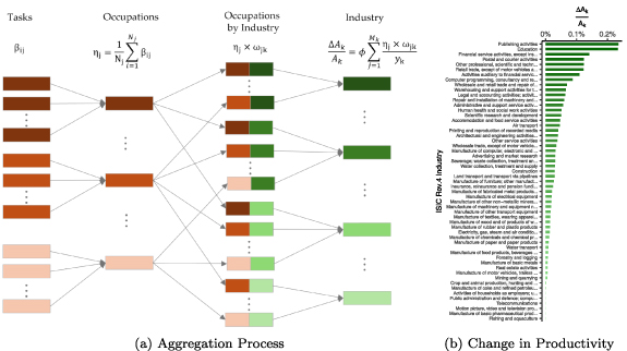
We begin with the exposure of tasks–specific activities or units of work performed within a job–to AI, β**ij. Exposure scores for 19, 265 tasks come from expert survey data from Eloundou et al [17]. AI exposure of each occupation is measured as the average of the AI exposure of its tasks. Occupational AI exposure is aggregated to the industry-level, measuring AI exposure for each of 55 industries as the average exposure of occupations within the industry weighted by their wage-bill share [18]. Finally, these AI exposure measures are merged with economic, energy, and emissions data for the US using the WIOD 2016 release and corresponding environmental accounts [20, 21]. This multi-step process allows us to consider not only which tasks are susceptible to AI, but also how important those tasks are within occupations, and how significant those occupations are within industries. It provides a comprehensive view of AI’s potential impact across the economy, linking granular task-level data to broad industry-wide effects.
We follow the approach of [22] to translate AI exposure to cost savings using a uniform scaling Cost Savings Factor, φ < 1, that is the product of two parameters: exposed tasks that are feasibly and profitably automated and the average fraction of labor cost savings for a task if AI is adopted. We follow [22] estimates that 23% of exposed tasks are profitably exposed tasks and that replacing human labor with AI results in 27% cost savings. This gives a Cost Savings Factor of  . Given their importance, we illustrate the sensitivity of our estimates to these parameters in figure 3.
We can then write the percentage change in productivity as
where, for industries k and occupations j, y is economic output, A is total factor productivity, φ is the Cost Savings Factor, η is the occupation-level exposure to AI, and ω is the wage-bill weight. The first identity follows from assuming that percentage changes in economic output are proportional to percentage changes in the productivity of the economy. That is, productivity affects all production inputs in the same proportion.
Putting this together, the right-hand panel of figure 1 shows estimates of the productivity impact of AI exposure across industries (see table A.3). We estimate a range of productivity impacts of AI from 0.233% for the education industry to 0% for industries like fishing and aquaculture.
To translate the economic productivity impacts of AI exposure to changes in energy use and carbon emissions we examine the relationships between industry-level productivity, energy intensity ν**k, and carbon intensity µ**k. Specifically, we calculate the change in economic output yk, the change in energy Ek, and the change in CO2 emissions Ck at the industry level as


Changes in output due to AI-driven productivity lead to a proportional increase in energy use, scaled by the industry’s energy intensity. And changes in energy use lead to a proportional increase in carbon emissions, scaled by the industry’s emissions intensity. Together, these equations allow us to trace the impact of AI-driven productivity changes on energy use and carbon emissions, accounting for the specific characteristics of each industry.
3.2. Industry-level impacts
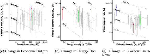
Figure 2 presents our main results for changes in output, energy use, and carbon emissions, corresponding to equations (2)–(4).
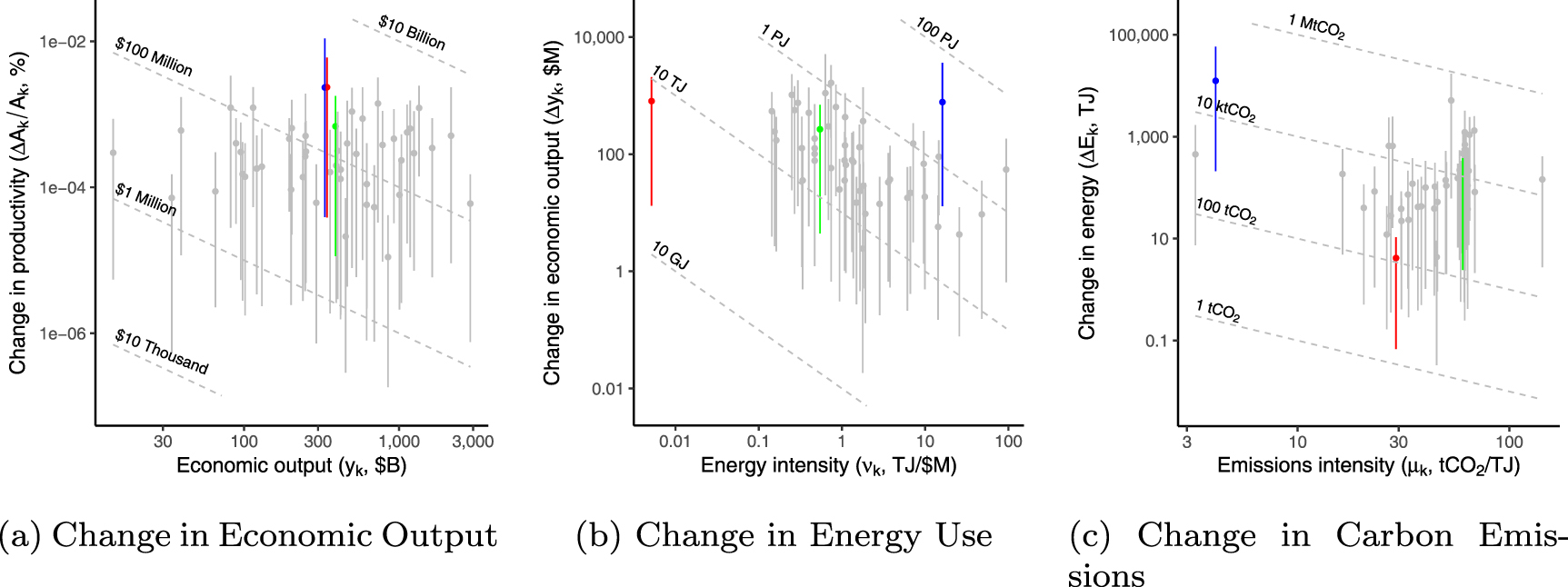
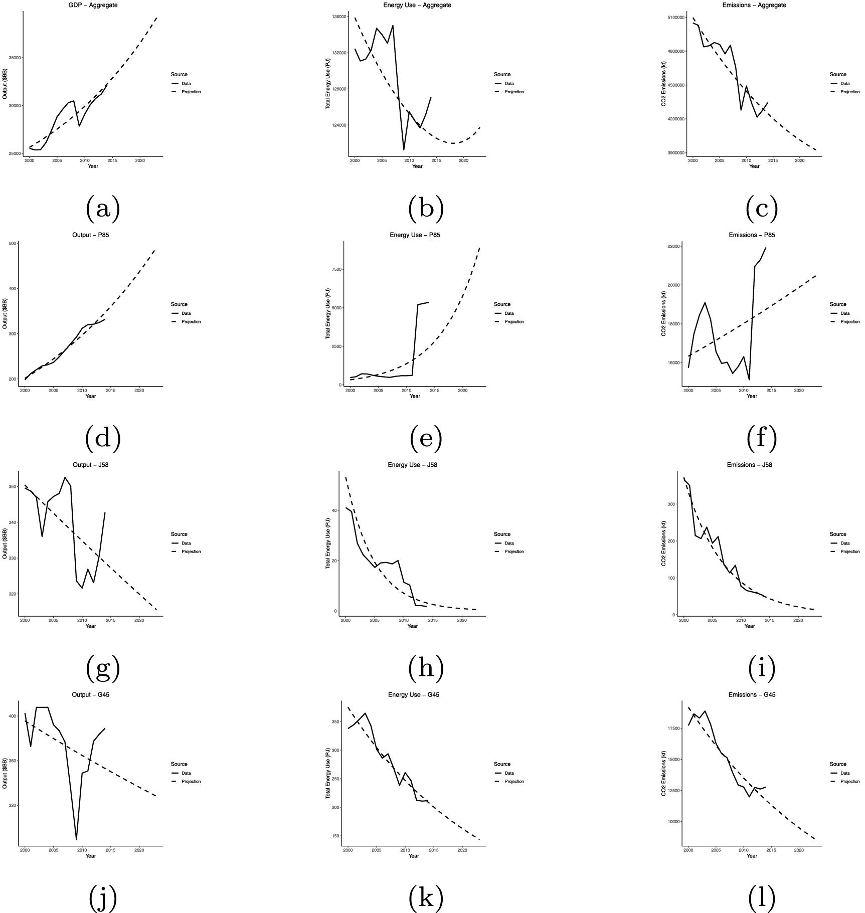
Figure 2. Impacts of AI by industry—the impact of AI adoption on (a) output, (b) energy use, and (c) CO2 emissions by industry. Each dot and whisker represents the estimates for a given industry where the dot represents our central estimates and the whiskers show the range of estimates across alternative assumptions regarding AI exposure rates from [17]. In color are ISIC Rev. 4 Codes P85:  , J58:
  , and G45:
 .
.
Download figure:
Standard image High-resolution image
On average, an industry in our study experiences a change in energy use of 0.511 petajoules (PJ) and a change in carbon emissions of 16 kilotons of CO2 (ktCO2). Yet, this average masks substantial variation across industries. Our estimates do not reveal a clear relationship between industry size and the magnitude of the AI-induced impact. Instead, the scale of impacts varies considerably–often across orders of magnitude.
The variation across industries stems from the structure of our model, which incorporates proportionality relationships between AI-driven changes in productivity and industry-specific characteristics. In general, smaller industries experience smaller absolute changes in output, less energy-intensive industries experience smaller changes in energy use, and less emissions-intensive industries experience smaller changes in carbon emissions.
To illustrate these patterns and the importance of capturing industry-level heterogeneity, table 1 summarizes the impacts for three distinct industries: Education, publishing activities, and Wholesale and retail trade and repair of motor vehicles and motorcycles. These industries are comparable in both initial economic output and estimated changes in productivity from AI adoption. Consequently, the change in economic output from AI is similar across these industries. However, differences in energy and emissions intensity lead to variation in how these productivity impacts from AI technologies translate into changes in energy use and emissions.
Table 1. The impact of AI on output (yk), energy use (Ek), and CO2 emissions (Ck) for selected industries.
| Industry | Change in productivity (%) | Industry size ($B) | Energy intensity (PJ/$B) | Emissions intensity (ktCO2 PJ−1) |  ($B) ($B) |  (PJ) (PJ) |  (ktCO2) (ktCO2) |
|---|---|---|---|---|---|---|---|
 | 0.233 | 332 | 16.13 | 4.10 | 0.774 | 12.477 | 51.133 |
  | 0.155 | 343 | 0.01 | 29.15 | 0.531 | 0.003 | 0.08 |
   | 0.076 | 389 | 0.54 | 60.29 | 0.296 | 0.161 | 9.711 |
For example, Education and Publishing have an initial economic output of just over $330B and experience similar estimated productivity increases, 0.0023%. This results in a comparable change in economic output of around $800M, as reflected in their similar vertical positions in figure 2(b). But, there is a spread in their energy intensities–16 TJ $M−1 for Education and 0.005 TJ $M−1 for Publishing Activities. This reflects differences in the dependence on energy as an input across industries, such as the energy-intensive nature of educational infrastructure. The differences in energy intensity lead to a divergence in the change in energy use following comparable changes in economic output–12PJ for Education and 0.004 PJ for Publishing Activities. This is reflected by a spread in their vertical positions in figure 3(c). Emissions intensity can introduce further divergence. Education has an emissions intensity of 4 tCO2 TJ−1 while Publishing Activities has a higher intensity of 29 tCO2 TJ−1. The mixture of energy sources powering economic production varies across industries, driving differences in emissions intensity. Taking the product of the change in energy use and emissions intensity, the change in emissions is 51 ktCO2 for Education and 0.1 ktCO2 for Publishing Activities.
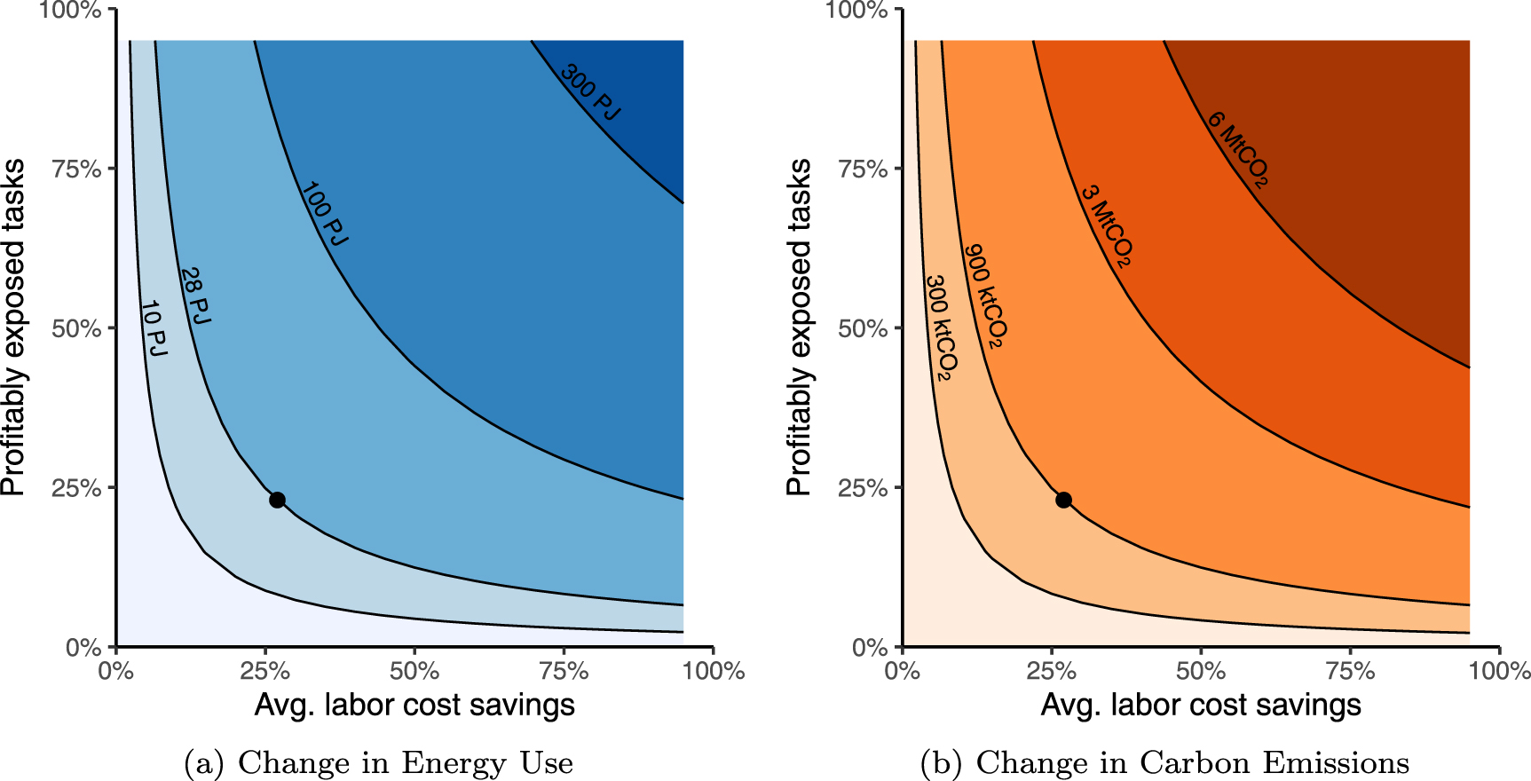
Figure 3. Sensitivity to Cost Savings Factor—sensitivity of (a) energy use and (b) carbon emissions estimates to alternative Cost Savings Factors. Cost Savings Factor is the product of the percentage of profitably exposed tasks and average percentage of labor cost savings, both bounded between 0% and 100%. The points represent the estimates presented in the text for the baseline Cost Savings Factor. Lines and colors highlight the gradients of how estimates change depending on the Cost Savings Factor.
Download figure:
Standard image High-resolution image 
This example underscores the importance of considering industry-specific characteristics in accurately assessing the energy and environmental impacts of AI adoption. Factors such as the current energy efficiency of an industry, the nature of its processes, and its capacity to integrate AI technologies all play important roles in determining the ultimate energy and emissions outcomes.
3.3. Aggregate impacts
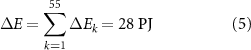
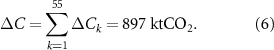
Aggregating across the 55 industry-specific impacts, the total annual change in energy use in the economy (ΔE) and in carbon dioxide emissions (ΔC) are given, respectively, as
As an aggregate change due to productivity gains from AI adoption, this first-order approximation encompasses the change in energy use across the whole economy, not just the energy required for training and running AI models.
So how does this compare to bottom-up estimates of the direct energy use of AI? For model training, the energy use of four widely used LLMs—BLOOM, GPT-3, Gopher, and OPT—ranged from 324 MWh to 1,287 MWh [4]. However, this is likely small compared to the ongoing energy expenditure for model inference. For instance, ChatGPT inference alone requires around 564 MWh per day or 0.2 Twh per year [4]. Yet, our estimate of 28 PJ (equivalent to about 7.8 TWh) per year is approximately 38 times larger than the annual energy use for ChatGPT inference.
We can also consider hardware-based estimates. NVIDIA, which holds a 95% market share, was expected to deliver 100, 000 AI servers in 2023. de Vries estimates that these servers, running at full capacity, consume approximately 5.7–8.9 TWh of electricity annually. Our estimate of 28 PJ (equivalent to about 7.8 TWh) suggests that the aggregate energy use from AI adoption is comparable to the direct electricity use of new hardware if run at full capacity, ranging from 88% to 137%. This indicates close alignment between our top-down and existing bottom-up estimates.
What does this change in energy use mean for generation capacity? An additional 28 PJ (or 7.8 TWh) per year implies that the US would require approximately 0.9 GW of additional generation capacity annually to keep up with the rising demand due to AI adoption-related productivity gains. This represents about 0.08% of the total US electricity generating capacity in 2021 (1,144 GW), indicating a relatively small but non-negligible impact on the national power infrastructure.
An increase of 897 ktCO2 emissions per year represents less than 1% of CO2 emissions from the US manufacturing and construction industries and is comparable to the annual emissions of a small country, like Iceland. In the context of the US, it accounts for approximately 0.02% of total CO2 emissions in 2021 (about 5 GtCO2), indicating that while the impact is measurable, it is a small fraction of overall emissions and thus will have minimal effect on climate change.
3.4. Sensitivity analysis
Our analysis above relies on a single estimate of the Cost Savings Factor derived from limited existing literature. Recognizing the uncertainty surrounding this crucial parameter, in figure 3 we perform a sensitivity analysis to set bounds on how variations in the Cost Savings Factor affect our estimates.
We illustrate the sensitivity of our estimates of the change in energy use (figure 3(a)) and change in carbon emissions (figure 3(b)) to the two measures that determine the Cost Savings Factor–the fraction of tasks that are profitably exposed to AI and the average labor cost savings for tasks performed by AI. Changes in both energy use and carbon emissions are bounded by the contribution of each industry to total economic output. This means that even in the most optimistic AI adoption scenarios—where cost savings and task exposure are at their highest—the changes in energy use and carbon emissions are still limited to a few percentage points of current levels.
These findings suggest that, while AI adoption may lead to increases in energy use and emissions, these increases are unlikely to be dramatically large relative to the overall economy, even under highly favorable conditions for AI. The sensitivity analysis also shows a non-linear relationship between cost savings, task exposure, and environmental impacts. Small changes in these parameters can lead to large changes in energy use and emissions, particularly in the middle ranges of the parameters. This underscores the importance of accurate estimates for these parameters and highlights areas where further research could significantly improve our understanding of AI’s energy and environmental impacts.
Our analysis provides a first (and first order) estimate of the impact of AI adoption on energy use and carbon emissions across the US economy. Here we highlight the assumptions and limitations inherent in our approach. We attempt to summarize and sign the expected effect on our estimates in table 2, distinguishing between the limitations of the modeling approach and those of the available data.
Table 2. The (plausible) effect of assumptions and data limitations on our estimates.
Overestimate (+)/Underestimate (−) Model Assumptions/Limitations
AI only affects productivity through labor− AI does not affect energy efficiency+ Prices and factors of production are fixed+/− No changes in the composition of the economy+/−
Data limitations
Only estimate of AI exposure comes from Eloundou et al [17]+/− Limited estimates and granularity for cost savings+/− Limited granularity of energy and environmental data+/− Energy and environmental data only through 2014+ Only consider impact in the US+/−
By assuming that AI only affects productivity by performing tasks previously performed by labor at a lower cost, we do not account for the possibility that AI could introduce new tasks or that AI could affect other forms of production, such as capital. By constraining the channels through which AI impacts productivity, we likely underestimate the aggregate impact of AI on productivity and, consequently, on energy use and carbon emissions.
Additionally, we focus on changes in energy use driven by productivity gains from AI adoption, ignoring the possibility of AI-driven improvements in energy efficiency. If AI were to spur improvements in energy efficiency, this would likely diminish the net impact of AI on energy use and carbon emissions, implying that our estimates would be overestimates.
Relatedly, our model assumes that prices and factors of production are fixed, so there are no changes in the composition of the economy. Thus, energy and emissions intensities are constant and there is no change in economic composition across industries. It is unclear a priori the sign of bias from these assumptions. It will likely depend on the relative energy and emissions intensities of growing and shrinking industries, and AI adoption could alter these factors over time.
Data availability also limits our analysis. While we consider alternative AI exposure measures, they all derive from a single dataset of AI exposure estimates [17]. Considering a broader range of exposure estimates could enhance the robustness of our findings, which could be done by applying our model to new estimates as they become available. This includes considering a broader array of AI technologies that could have different implications for productivity and energy impacts.
Another key data limitation is the varying granularity of data. Ideally, we would have all relevant data at the task level. However, while data on AI exposure is available at the task level, energy and carbon data are at the industry-level and we apply a single uniform Cost Savings Factor. Finer granularity will improve the accuracy of our estimates but it is not obvious the sign of any bias from aggregation.
For our analysis, we measure energy intensity and carbon intensity using data for 2014 to be consistent with the most recent economic data in WIOD. Yet, there has been a trend towards improved energy efficiency and decarbonization of energy systems in the US. By using older data, we likely overestimate the impact of AI on energy use and carbon emissions. In the appendix B, we project output, energy use, and emissions through 2023 and re-estimate the impact of AI. We find changes in energy use and carbon emissions decrease slightly to 24PJ and 790ktCO2, respectively. This minimal change after a decade of increases in energy efficiency and decarbonization suggests it would take a large, non-linear change in energy efficiency improvements or decarbonization to fundamentally change our results. Likely, the only way for this to occur is through stringent energy and climate policy, such as an even stronger push towards electrification paired with decarbonization of electricity generation than we have seen in the recent past.
Related, we do not have information on the spatial distribution of energy use, which could have implications for the estimated change in carbon emissions as the emissions intensity of energy varies across regions, both within the US and beyond. In the case of our analysis, near-term capital and political constraints are likely to prevent any significant changes in the regional distribution of energy use. That is, within industries, production and sources of energy are unlikely to change very much, though the balance between industries may change as they grow at different rates. Yet, future changes in the distribution of economic production, energy use, and sources of power generation, such as a shift to renewable energy generation, could affect the overall carbon emissions impacts of AI. This is also the case if we consider the implications of our analysis beyond the scope of the United States. Starting with the economic impact, our estimates indicate a relatively larger impact of AI on services-based industries than in manufacturing or agriculture industries. This is due to both the type of tasks performed in these industries and that we only consider impacts through labor, which is a larger share of costs for service-based industries. Thus, in countries with higher proportion of manufacturing or agriculture industries relative to services than in the US, the expected economic gains, and thus changes in energy and emissions, would be smaller. Similarly, energy intensity of production and emissions intensity of energy varies across countries. A given change in energy use will lead to a greater increase in emissions in a low-carbon economy like Norway with high use of renewable energy generation than in a country like South Africa with a high amount of coal power generation. A global analysis could apply our methodology to provide a more comprehensive picture of AI’s impact on energy use and emissions.
Through our parsimonious model, we capture both the direct and indirect effects of AI adoption across the economy. This provides a more comprehensive view of AI’s potential impact on energy use and emissions than approaches focusing solely on the energy consumption of AI hardware or specific AI applications. Our findings indicate that, while AI adoption does increase energy use and emissions, the magnitude of this increase is relatively modest compared to overall economic activity. However, the cumulative effect over time and across industries underscores the importance of considering energy and environmental impacts in AI development and deployment strategies. Moreover, the variation in impacts across industries highlights the need for industry-specific approaches to managing the energy and environmental consequences of AI adoption.
As AI continues to transform various industries of the economy, we must balance productivity gains and economic benefits with potential increases in energy demand and associated carbon emissions. This may involve prioritizing energy-efficient AI technologies, investing in renewable energy sources to power AI infrastructure, and developing strategies to offset increased emissions in AI-intensive industries. It may also involve prioritizing efforts to leverage AI to mitigate vulnerabilities to climate change by increasing resilience to climate stressors, such as increased extreme weather events.
Future research could address some of the limitations identified here, incorporating dynamic effects, exploring industry-specific AI impacts, and investigating the interplay between AI-driven productivity gains and energy efficiency improvements. Such work would further refine our understanding of AI’s role in shaping future energy demand and environmental outcomes. Additionally, as more data becomes available on the real-world impacts of AI adoption across different industries, researchers can update and refine the estimates presented in this study.
It is also worth considering the potential for AI itself to contribute to solutions for energy efficiency and emissions reduction. AI technologies could play a significant role in optimizing renewable energy sources, such as wind and solar power. AI can also optimize industrial processes, increasing overall efficiency and reducing waste. Future studies should consider these aspects to provide a more comprehensive view of AI’s environmental impact.
In conclusion, our study provides a valuable starting point for understanding the broader energy and environmental implications of AI adoption across the economy. We hope to stimulate further research and informed discussion on this important topic by highlighting both the potential impacts and the areas of uncertainty. As AI continues to evolve and reshape various aspects of our economy and society, ongoing analysis and monitoring of its energy and environmental impacts will ensure sustainable development of these transformative technologies.
The data that support the findings of this study are openly available at the following URL/DOI: https://doi.org/10.7910/DVN/ZHKD3X.
A R H and J M C were supported by funding from Google. The funder had no role in the design, analysis, interpretation, or writing of this paper. All findings and conclusions are solely those of the authors.
Here we show the complete list of impacts by industry.
Table A.3. Changes in GDP, energy, and emissions by industry.
| Industry | Code | Change in GDP | Change in Energy | Change in Emissions |
|---|---|---|---|---|
| Fishing and aquaculture | A03 | 0 | 0 | 0 |
| [0, 0] | [0, 0] | [0, 0] | ||
| Public administration and defense | O84 | 0 | 0 | 0 |
| [0, 0] | [0, 0] | [0, 0] | ||
| Activities of households as employers | T | 0 | 0 | 0 |
| [0, 0] | [0, 0] | [0, 0] | ||
| Manufacture of coke and refined petroleum | C19 | 0.009 40 | 0.450 08 | 1.480 14 |
| [0.000 15, 0.035 26] | [0.007 41, 1.689 08] | [0.024 36, 5.554 75] | ||
| Crop and animal production | A01 | 0.009 58 | 0.018 30 | 1.127 24 |
| [0.000 13, 0.032 08] | [0.000 25, 0.061 26] | [0.015 35, 3.773 19] | ||
| Mining and quarrying | B | 0.036 96 | 0.139 69 | 6.991 16 |
| [0.000 53, 0.138 86] | [0.002 01, 0.524 87] | [0.100 43, 26.269 15] | ||
| Manufacture of motor vehicles | C29 | 0.035 65 | 0.012 03 | 0.317 06 |
| [0.000 49, 0.128 59] | [0.000 17, 0.043 39] | [0.004 39, 1.143 55] | ||
| Real estate activities | L68 | 0.172 19 | 0.028 01 | 0.771 74 |
| [0.002 19, 0.433 98] | [0.000 36, 0.070 60] | [0.009 81, 1.945 05] | ||
| Manufacture of basic metals | C24 | 0.017 94 | 0.109 80 | 6.973 84 |
| [0.000 21, 0.060 19] | [0.001 31, 0.368 31] | [0.082 92, 23.393 44] | ||
| Manufacture of chemicals | C20 | 0.039 83 | 0.382 78 | 10.323 34 |
| [0.000 77, 0.140 94] | [0.007 43, 1.354 46] | [0.200 33, 36.528 83] | ||
| Forestry and logging | A02 | 0.002 45 | 0.004 35 | 0.197 36 |
| [0.000 02, 0.005 12] | [0.000 03, 0.009 11] | [0.001 49, 0.413 30] | ||
| Manufacture of food products | C10_12 | 0.079 21 | 0.104 58 | 4.655 48 |
| [0.002 13, 0.231 78] | [0.002 81, 0.306 02] | [0.125 28, 13.622 78] | ||
| Water transport | H50 | 0.005 74 | 0.082 02 | 5.634 90 |
| [0.000 15, 0.019 64] | [0.002 13, 0.280 77] | [0.146 01, 19.289 56] | ||
| Manufacture of paper and paper products | C17 | 0.018 69 | 0.185 12 | 3.015 34 |
| [0.000 49, 0.057 33] | [0.004 88, 0.567 80] | [0.079 55, 9.248 73] | ||
| Manufacture of basic pharmaceutical products | C21 | 0.028 60 | 0.014 26 | 0.129 63 |
| [0.000 58, 0.106 96] | [0.000 29, 0.053 31] | [0.002 65, 0.484 72] | ||
| Electricity, gas, steam and air conditioning supply | D35 | 0.054 58 | 5.132 49 | 272.831 47 |
| [0.000 65, 0.183 54] | [0.061 28, 17.260 50] | [3.257 36, 917.528 20] | ||
| Manufacture of wood and wood products | C16 | 0.014 16 | 0.040 15 | 0.824 26 |
| [0.000 18, 0.040 89] | [0.000 51, 0.115 96] | [0.010 41, 2.380 56] | ||
| Manufacture of rubber and plastic products | C22 | 0.034 60 | 0.124 68 | 4.348 24 |
| [0.000 69, 0.108 25] | [0.002 48, 0.390 05] | [0.086 41, 13.603 02] | ||
| Telecommunications | J61 | 0.099 17 | 0.011 04 | 0.540 65 |
| [0.002 65, 0.242 68] | [0.000 29, 0.027 02] | [0.014 42, 1.323 05] | ||
| Manufacture of textiles | C13_15 | 0.014 86 | 0.022 20 | 0.686 90 |
| [0.000 27, 0.040 85] | [0.000 41, 0.061 04] | [0.012 66, 1.888 51] | ||
| Manufacture of other transport equipment | C30 | 0.057 93 | 0.042 94 | 1.647 89 |
| [0.000 67, 0.220 11] | [0.000 50, 0.163 13] | [0.019 08, 6.261 22] | ||
| Manufacture of machinery and equipment n.e.c. | C28 | 0.073 40 | 0.100 64 | 4.045 01 |
| [0.000 76, 0.243 58] | [0.001 04, 0.334 00] | [0.041 68, 13.423 78] | ||
| Manufacture of other non-metallic mineral products | C23 | 0.021 79 | 0.144 73 | 20.723 46 |
| [0.000 41, 0.061 82] | [0.002 74, 0.410 61] | [0.392 90, 58.794 07] | ||
| Manufacture of electrical equipment | C27 | 0.024 98 | 0.023 35 | 0.781 01 |
| [0.000 31, 0.082 70] | [0.000 29, 0.077 31] | [0.009 62, 2.585 39] | ||
| Manufacture of fabricated metal products | C25 | 0.078 13 | 0.083 93 | 1.937 80 |
| [0.001 03, 0.240 34] | [0.001 10, 0.258 18] | [0.025 43, 5.961 08] | ||
| Insurance, reinsurance and pension funding | K65 | 0.242 35 | 0.037 63 | 2.392 46 |
| [0.002 69, 0.548 19] | [0.000 42, 0.085 12] | [0.026 58, 5.411 71] | ||
| Manufacture of furniture | C31_32 | 0.064 11 | 0.071 42 | 2.370 54 |
| [0.000 92, 0.188 17] | [0.001 02, 0.209 63] | [0.033 91, 6.957 53] | ||
| Motion picture, video and television programme production | J59_60 | 0.090 06 | 0.001 66 | 0.046 84 |
| [0.001 79, 0.233 83] | [0.000 03, 0.004 30] | [0.000 93, 0.121 63] | ||
| Land transport and transport via pipelines | H49 | 0.152 01 | 1.091 09 | 70.795 56 |
| [0.003 12, 0.336 45] | [0.022 40, 2.415 03] | [1.453 69, 156.698 77] | ||
| Construction | F | 0.365 89 | 0.656 34 | 18.442 84 |
| [0.009 01, 1.379 06] | [0.016 16, 2.473 80] | [0.454 04, 69.512 71] | ||
| Water collection, treatment and supply | E36 | 0.004 26 | 0.109 49 | 5.522 49 |
| [0.000 08, 0.012 38] | [0.002 01, 0.318 14] | [0.101 17, 16.046 10] | ||
| Sewerage; waste collection, treatment and disposal activities | E37_39 | 0.028 95 | 0.052 31 | 2.392 45 |
| [0.000 51, 0.073 35] | [0.000 92, 0.132 53] | [0.042 13, 6.061 64] | ||
| Advertising and market research | M73 | 0.077 45 | 0.036 41 | 2.142 77 |
| [0.001 23, 0.204 12] | [0.000 58, 0.095 95] | [0.034 01, 5.647 12] | ||
| Manufacture of computer, electronic and optical products | C26 | 0.126 72 | 0.041 83 | 1.546 58 |
| [0.001 18, 0.437 69] | [0.000 39, 0.144 50] | [0.014 42, 5.342 11] | ||
| Wholesale trade, except of motor vehicles and motorcycles | G46 | 0.535 26 | 0.144 32 | 8.801 61 |
| [0.009 14, 1.365 41] | [0.002 46, 0.368 15] | [0.150 27, 22.452 40] | ||
| Other service activities | R_S | 0.297 47 | 0.204 67 | 12.276 41 |
| [0.007 51, 0.866 50] | [0.005 17, 0.596 19] | [0.309 96, 35.759 97] | ||
| Architectural and engineering activities | M71 | 0.184 70 | 0.086 82 | 5.109 78 |
| [0.002 02, 0.711 20] | [0.000 95, 0.334 31] | [0.055 84, 19.675 46] | ||
| Printing and reproduction of recorded media | C18 | 0.035 60 | 0.038 36 | 1.182 87 |
| [0.002 81, 0.078 18] | [0.003 02, 0.084 25] | [0.093 27, 2.597 95] | ||
| Air transport | H51 | 0.090 41 | 1.316 83 | 89.964 91 |
| [0.009 08, 0.173 30] | [0.132 28, 2.524 23] | [9.037 02, 172.454 41] | ||
| Accommodation and food service activities | I | 0.428 64 | 0.468 34 | 28.281 31 |
| [0.029 84, 1.091 79] | [0.032 60, 1.192 92] | [1.968 59, 72.035 82] | ||
| Scientific research and development | M72 | 0.125 93 | 0.059 20 | 3.484 01 |
| [0.001 40, 0.477 04] | [0.000 66, 0.224 24] | [0.038 73, 13.197 45] | ||
| Human health and social work activities | Q | 1.101 39 | 0.696 61 | 42.947 67 |
| [0.019 81, 5.073 54] | [0.012 53, 3.208 89] | [0.772 42, 197.837 39] | ||
| Administrative and support service activities | N | 0.637 64 | 0.540 30 | 33.770 95 |
| [0.019 14, 1.532 23] | [0.016 22, 1.298 32] | [1.013 68, 81.150 48] | ||
| Repair and installation of machinery and equipment | C33 | 0.023 57 | 0.038 84 | 1.717 06 |
| [0.000 46, 0.067 43] | [0.000 76, 0.111 14] | [0.033 43, 4.913 06] | ||
| Legal and accounting activities | M69_70 | 0.751 34 | 0.222 07 | 12.938 69 |
| [0.012 94, 1.824 27] | [0.003 82, 0.539 19] | [0.222 77, 31.415 52] | ||
| Warehousing and support activities for transportation | H52 | 0.131 51 | 0.213 78 | 13.736 76 |
| [0.004 59, 0.319 97] | [0.007 46, 0.520 16] | [0.479 50, 33.423 12] | ||
| Wholesale and retail trade and repair of motor vehicles | G45 | 0.295 78 | 0.161 05 | 9.710 64 |
| [0.004 88, 0.769 03] | [0.002 66, 0.418 74] | [0.160 23, 25.247 86] | ||
| Computer programming, consultancy and related activities | J62_63 | 0.592 54 | 0.237 04 | 14.645 65 |
| [0.007 40, 1.579 59] | [0.002 96, 0.631 90] | [0.182 81, 39.042 09] | ||
| Activities auxiliary to financial services and insurance | K66 | 0.541 75 | 0.077 90 | 4.772 60 |
| [0.003 91, 1.143 07] | [0.000 56, 0.164 37] | [0.034 48, 10.069 97] | ||
| Other professional, scientific and technical activities | M74_75 | 0.100 90 | 0.047 43 | 2.791 47 |
| [0.002 30, 0.275 84] | [0.001 08, 0.129 66] | [0.063 52, 7.631 16] | ||
| Postal and courier activities | H53 | 0.141 06 | 0.153 54 | 8.765 02 |
| [0.006 15, 0.270 75] | [0.006 69, 0.294 71] | [0.382 15, 16.823 53] | ||
| Retail trade, except of motor vehicles and motorcycles | G47 | 1.726 90 | 1.279 43 | 78.779 55 |
| [0.193 33, 3.492 53] | [0.143 24, 2.587 57] | [8.819 53, 159.326 42] | ||
| Financial service activities, except insurance | K64 | 1.027 93 | 0.256 78 | 16.180 83 |
| [0.024 14, 2.325 56] | [0.006 03, 0.580 94] | [0.380 04, 36.606 99] | ||
| Publishing activities | J58 | 0.531 42 | 0.002 74 | 0.079 93 |
| [0.007 26, 1.367 13] | [0.000 04, 0.007 05] | [0.001 09, 0.205 64] | ||
| Education | P85 | 0.773 59 | 12.477 47 | 51.133 27 |
| [0.012 98, 3.618 02] | [0.209 43, 58.355 91] | [0.858 26, 239.145 26] |
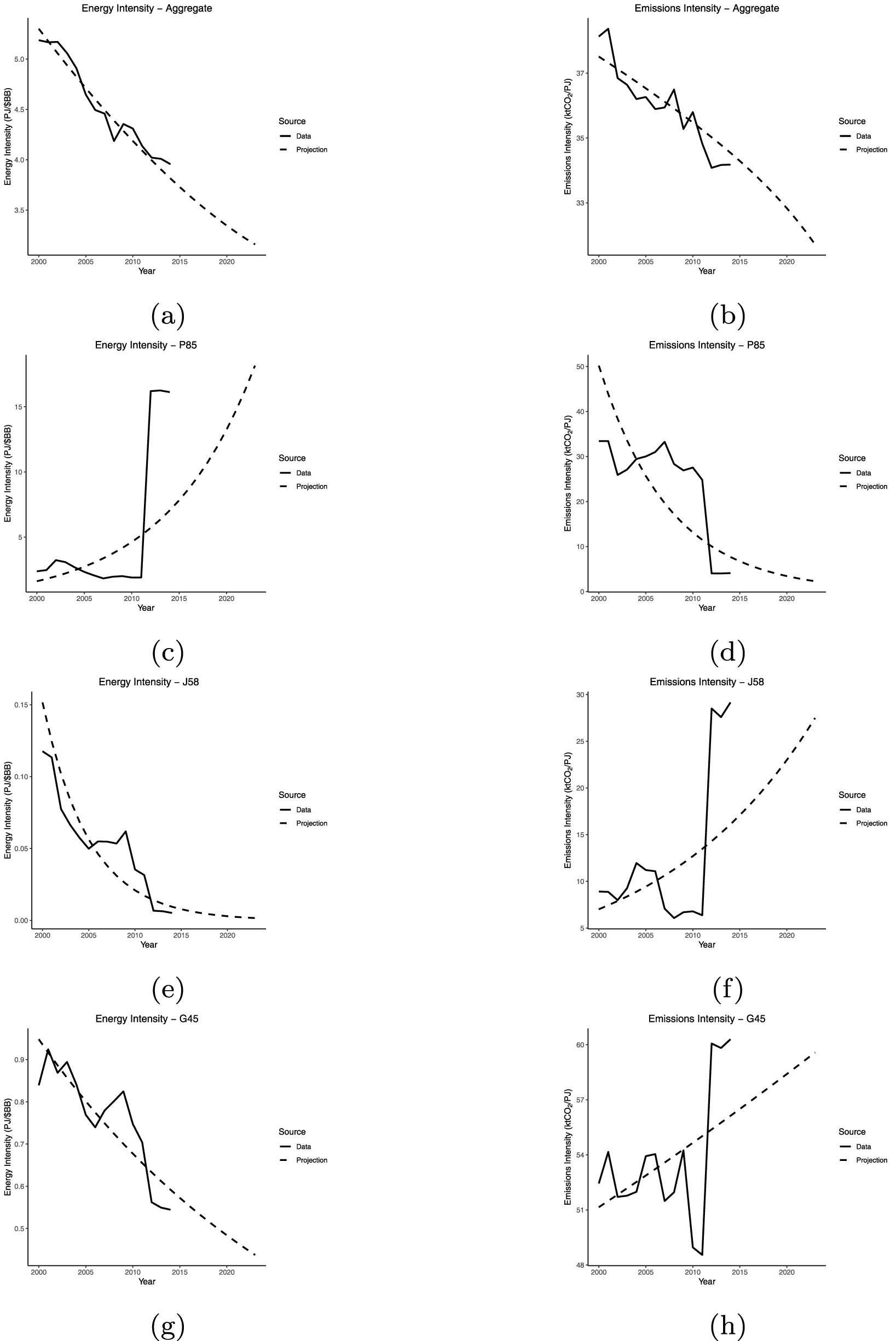
For data on energy use and emissions at the industry level, we use the Environmental Accounts from the WIOD 2016 release’s corresponding Environmental Accounts. These data cover the years 2000–2016. For our analysis in the text, we use data for the year 2014 since it is the most recent year of economic data available. However, using older data potentially introduces bias in our analysis (table 2). Specifically, energy intensity and emissions intensity change over time, on the aggregate level generally declining with time (figures B.5(a) and (b)). This suggests that using more recent data on energy and emissions would lead to lower estimates for the energy and emissions impact of changes in productivity due to AI adoption.
To get at the potential scale of this bias, we use a simple projection of industry-level output, energy use, and emissions. For each industry and variable, we fit a log-linear curve to the data from 2000 to 2014 and use this fit to project the variable out to 2023 (figure B.4). We then use the projected values to recalculate industry-level energy intensity and emissions intensity (figure B.5). Finally, we use the projected values for 2023 to recalculate the impact of AI adoption on energy use and CO2 emissions.
Figure B.4. Projection of output, energy use, and emissions.
Download figure:
Standard image High-resolution image 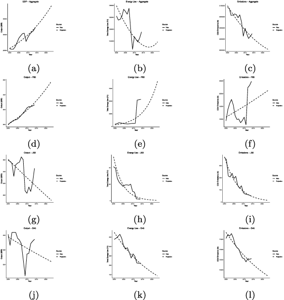
Figure B.5. Projection of energy intensity and emissions intensity.
Download figure:
Standard image High-resolution image 
Using the new projected values for industry-level energy intensity and emissions intensity we recalculate the aggregate change