1748-9326/20/11/114075

Abstract

Floods and droughts create temporal disconnects between water supply and demand, underscoring the need to store high magnitude flows (HMFs) in depleted aquifers to alleviate these extremes. The objective of this study was to quantify the spatial and temporal variability of HMFs to inform managed aquifer recharge (MAR), accounting for water rights, instream flow requirements, and coastal inflows. Texas, USA, was selected as the study area due to its climate-driven water stress, rising water demand, and the availability of detailed data on legal constraints. Volumes of HMFs (defined as ⩾ 95th percentile) were calculated for 190 streamflow monitoring gages in all 23 river basins in Texas (1968–2022). Water availability models and coastal inflow requirements were used to consider limitations to HMF availability for permitted use, including water rights, environmental flows, and coastal inflows for select major river basins. Results show that HMFs averaged 31% of total flows across all stations in the state. Of these HMFs, 52% of flows were unappropriated (not reserved for water rights holders), representing 12% of total flows. The mean annual volume of unappropriated HMFs was 81 Mm3 (∼0.07 million acre-feet). Mean annual unappropriated HMF volumes increased by a factor of 100 from semi-arid West Texas to humid southeast Texas, with variability driven by basin climate and watershed size. Environmental flow requirements generally did not significantly reduce the unappropriated HMFs as they were accommodated by flow reserved for downstream senior water rights. However, coastal inflow requirements limited permittable HMF volumes, especially in the semiarid Colorado River basin which includes high urban water demand up-basin. When considering volumes of HMFs that may be considered ‘available’, it is essential to consider limitations to the amount of flows that could be permitted. This study provides a template for assessing HMFs for MAR that considers water rights, environmental flows, and coastal inflow requirements that could be generally applied in many regions (particularly the western US) to address climate extremes.

Export citation and abstractBibTeXRIS

Increasing climate extremes (floods and droughts) are challenging water managers globally because they drive excessive amounts of water when it is not needed, and a shortage when it is needed. Temporal disconnects between excess water supply and demand result in adverse economic and environmental impacts from floods and droughts. These disconnects underscore the importance of capturing and storing excess water when it is available, partially resolving these disconnects. Many semi-arid regions, such as the western US and Australia, experience prolonged droughts that are interrupted by intense drought-ending flood events, resulting in marked variability in water supplies over time [1–3]. Storing water is typically done using surface water reservoirs; however, evaporative losses from surface water bodies are increasing globally at a rate of ∼3.1 km3 yr−1 [4]. There is increasing interest in storing excess surface water flows in depleted aquifers to minimize evaporative losses [5–7]. There is an estimated 1,000 km3 of storage space in depleted aquifers in the US, which exceeds the surface reservoir capacity of 673 km [3, 8, 9], indicating substantial storage space in certain aquifers [10]. These depleted aquifers are often located in semi-arid climates in the western US [6] where water scarcity is a critical issue [11].

High magnitude flows (HMFs) refer to flows that occur within a stream channel and/or floodplain during or immediately following a storm event [12]. Threshold flows of 90th and 95th percentile streamflows have been used to define HMFs [13, 14]. HMFs are being explored as a cost-effective way to artificially replenish groundwater via managed aquifer recharge (MAR) given that infrastructure and energy requirements for capture are lower than those for desalination or municipal wastewater treatment [15–17]. MAR, including surface spreading basins and injection wells aquifer storage and recovery (ASR), is sometimes referred to interchangeably as enhanced aquifer recharge, and is defined by the U.S. Environmental Protection Agency as intentional recharge of aquifers to provide water supply or environmental benefits [17]. Sources for MAR can include HMFs, treated wastewater, and desalinated water. This practice has been implemented to alleviate water scarcity along with other benefits including flood mitigation, land subsidence, and saltwater intrusion [18].

In areas worldwide where prolonged droughts, periodic flooding, and demand for water resources all intersect, the use of excess flows for enhancing aquifer recharge has emerged as an innovative method of addressing increasing water scarcity [13, 19, 20]. The feasibility of MAR projects depends on the overall cost-benefit of implementation [18, 21, 22]. Prior research suggests that groundwater storage can provide six times more storage capacity than surface reservoirs for the same cost [21], and large-scale MAR operations can have a favorable cost-benefit ratio [7, 23, 24]. MAR has been implemented using several different techniques across multiple geographies with the primary goal of addressing water security [19, 24] (figure 1). Although MAR storage (∼10 km3 yr−1) is much less than that of surface reservoirs (7,000–8,300 km3) globally, MAR represents an important component of a portfolio of strategies to manage water resources locally [20]. MAR takes advantage of the long-term storage capability of aquifers with the added benefits of high storage capacity, minimal land requirements, and minimal evaporative losses [6].

Figure 1. Examples of different HMF-based MAR techniques applied across a range of different climatic and water use scenarios throughout the continental US. This includes intentional flooding of orchards in Central Valley of California to promote infiltration [25], routing excess surface flows to an infiltration basin in the Arizona desert [26, 27], injecting excess river flows into an injection well in the Florida Everglades [28], and re-routing an ephemeral stream into a sinkhole to recharge a karst aquifer in Texas[29]. Major principal aquifers are shown as transparent grey polygons and represent the potential areas of HMF storage where aquifers are depleted. The climatic gradient, shaded by the average annual precipitation for 1991–2020 [30], indicates the wide array of precipitation regimes across the US, and specifically Texas. (Top left) Photo credit: Helen Dahlke. (Bottom left) Reproduced with permission from Central Arizona Project [27]. (Top right) Reproduced with permission from USACE [28]. (Middle) Reproduced with permission from PRISM Group [30]. Copyright ©2025, PRISM Group, Oregon State University, https://prism.oregonstate.edu Map created 1 February, 2025. (Bottom right) Photo credit: Marcus Gary, 2015.

Download figure:

Standard image High-resolution image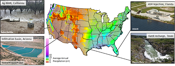

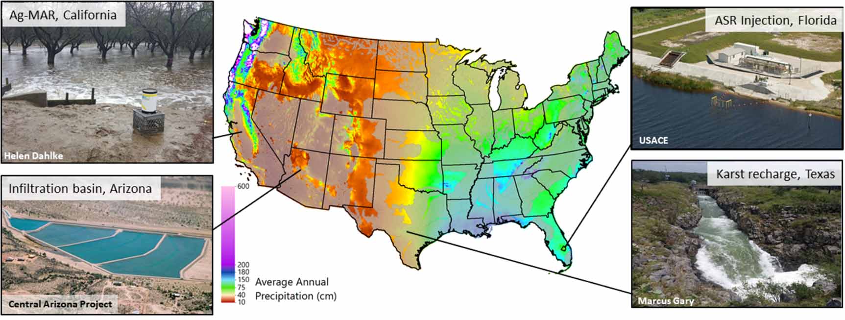
For HMFs to be considered potentially accessible for MAR, legal restrictions on water capture (including water rights, environmental flow requirements, and coastal inflows) need to be considered and permitted by the appropriate legal bodies, such as the Texas Commission on Environmental Quality (TCEQ) in Texas, USA. Surface flows are allocated to water rights users for many purposes (municipal, agricultural, industrial, etc), resulting in the fraction of surface flows that are potentially accessible for MAR being highly variable and dependent on site-specific legal and environmental considerations [12]. These constraints create multiple ‘levels’ of potential availability that are considered in the permitting process (figure 2(a)).

Figure 2. (a) there are multiple levels to ‘availability’ of HMFs: 1) the flow must be an HMF, defined here as a flow exceeding the 95th percentile; 2) the flow has to also be unappropriated (not allocated for a water rights permit holder); 3) the flow must exceed instream flow targets; 4) the flow must exceed coastal inflow targets; and 5) most importantly, the flow can only be considered available for actual use by securing water use permits by the appropriate permitting/governing bodies. (b) A flowchart depicts the analyses conducted in this study to estimate the levels of potential HMF availability in Texas, including the USGS streamflow datasets and water availability models, water usage scenarios (full-use assumes all allocated water is used by water rights holders and no return flows, and current-use is a best estimate of actual water usage including return flows), instream flow targets, and coastal inflow targets.

Download figure:

Standard image High-resolution image

Water rights accounting varies between the western and eastern US due to differences in climate, history, and land ownership [31]. Western states, including Texas, generally implement a doctrine of prior appropriation (the ‘first in time, first in right’ approach) while eastern states typically follow the riparian doctrine, where one must own land next to the watercourse and extract a reasonable amount of water defined by the state [32]. Water rights accounting can be estimated in Texas using publicly available data, and can provide a template for other regions that have similar legal schema.

Environmental flows are defined as a portion of surface flows, including the timing, magnitude, and quality of flows, required to maintain healthy stream ecology [12, 33, 34]. Environmental flow standards address the protection of instream flows, referring to stream flows at inland locations, and freshwater inflows into coastal bays and estuaries, hereafter referred to as coastal inflows.

Instream flow standards are an active area of research and have been estimated using a variety of approaches, often requiring 20% to 80% of mean annual stream flows to be preserved [33–37]. Environmental flows were originally intended to maintain natural variability in stream flows, particularly minimum flows that limit disruption by river damming and extraction for water supplies [33, 38]. High flows were also found to be essential to riparian health by moving sediments and improving water quality and connectivity, resulting in a certain portion of high flows being reserved for this purpose [12, 39]. Data for both water rights and environmental flows are limited, with different terminology, legal frameworks, and data access protocols among states [40]. California, for example, has major gaps in data availability and different water rights regimes for certain river basins and groundwater systems (i.e. adjudicated basins [41]).

Coastal inflow standards are intended to protect the volume of freshwater inflows necessary to maintain normal estuarine functions [42]. Methodologies for determining, adjudicating, and monitoring coastal inflows are complex given the site-specific needs of coastal systems [43]. The relationship between freshwater inflows and salinity provide the foundation for management targets, as key ecosystem processes and associated ecosystem services are modulated by this relationship [42, 44]. Areas where coastal inflows are adjudicated separately from instream flows include San Francisco Bay, bays and estuaries in Texas, and southern Florida (USA), Australia, and South Africa [44, 45]. Texas has implemented an adaptive management system that includes bay-specific coastal inflow standards to ‘maintain salinity, nutrient, and sediment loading regimes intended to support an ecologically sound environment in the receiving bay and estuary system’ [42, 44, 45]. These requirements increase the complexity of assessing permittable HMF volumes that could potentially be used for MAR.

The objective of this study was to take a first step in quantifying the levels of historical HMF ‘availability’ including constraints related to water rights, environmental flows (instream flow targets (IFT); and coastal inflows) using Texas as a case study (figure 2(b)). These constraints were neglected in previous studies [13, 14]. Although the quantities discussed in this study do not include the complete legal mechanisms considered by the TCEQ during the water use permitting process, they represent key limitations to what portion of HMFs could actually be considered ‘available’.

Wurbs [46] developed Water Availability Models (WAMs) for all 23 river basins in Texas to quantify water appropriations and resultant unappropriated flows at a monthly timestep. Wurbs [47] also developed daily timestep WAMs that include instream flow requirements for three of the largest river basins by area and discharge—the Colorado, Brazos, and Trinity Rivers—covering 38% of the area of Texas. These models allow for event-scale budgeting of unappropriated flows during high flow events. By pairing these WAMs with stream gage data from the United States Geological Survey (USGS), HMF availability was estimated for 190 stations in Texas. Unique aspects of this study include:

(a)

descriptive HMF statistics throughout river basins

(b)

estimation of unappropriated HMFs considering water rights using statewide WAMs

(c)

estimation of HMF availability for MAR considering water rights and instream flows for three large river basins, and

(d)

reconnaissance-level analysis of coastal inflow requirements for these three large river basins (figure 2(b)).

Previous studies estimated HMFs for MAR, but did not consider water rights or instream flows [14] or only accounted for water rights at river basin outlets [13]. We built on these efforts by including water rights at 190 gage stations statewide, and additionally considering environmental flows for select large river basins (figure 2(b)). This allowed for a comparison of multiple climatological and water rights scenarios.

We focused on Texas as it is subjected to extreme flows (both floods and prolonged droughts), has depleted aquifers, and a rising population that routinely places stress on water resources. Texas population is projected to grow from 29.5 million (2020) to 51 million (2070) with corresponding increase in water demand from 21.8 km3 (17.7 million acre-feet, maf, 2020) to 23.7 km3 (19.2 maf, 2070) [48]. A strong climatic gradient from east (humid) to west (semi-arid) drives variation in water stress across the state [49]. Texas lies in the central portion of the greater climate gradient that spans humid eastern US to semiarid western US, divided by the 100th meridian (figure 1). Precipitation is characterized by prolonged droughts interrupted by irregular intense rain events [50–52]. This variability requires increased storage to manage climate extremes. The approach for estimating availability of HMFs applied in Texas can provide a template for other regions similarly impacted by water stress.

2.1. Texas river basins

There are 23 river basins in Texas, including 15 major basins and 8 coastal basins between the major basins (figure 3(a)). Most river basins drain into the Gulf of Mexico by way of coastal estuaries or direct discharge, except four (Canadian, Red, Sulphur, and Cypress) which drain eastward into the Mississippi River basin. The Rio Grande River was not included given the complexity of international water treaties and lack of WAM model control points on the main stem of the river.

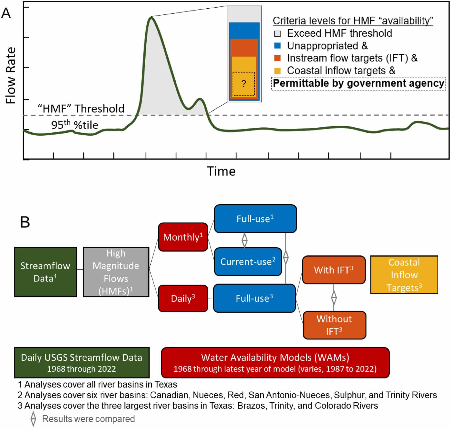
Figure 3. (a) Study area map showing the major river basins of Texas, and the selected WAM control points that are associated with USGS stream gages and include the variables of interest for the accounting of HMF (unappropriated flows for monthly WAMs; both unappropriated flow and instream flow targets for daily WAMs). (b) Map of the mean annual HMF volume for each station for the period 1968–2022, colored and sized by volume in million cubic meters (Mm3), (c) scatter plot of the mean annual HMF volumes relative to watershed area, and (d) a 3D plot showing the non-linear relationship between average storm duration, storm frequency, and HMF volume for each station.

Download figure:

Standard image High-resolution image

2.2. USGS gage data

Descriptive HMF statistics were based on daily mean streamflow for 55 years (1968–2022) from 206 stations covering all 23 river basins (figure S1). To maximize data consistency, stations lacking five consecutive years of data were omitted. A year was considered missing if it had < 310 daily records.

HMF metrics were calculated following the methods from previous studies [13, 14]. These studies used either the 95th and 90th percentiles of daily mean flows for each gage as the threshold beyond which flows are considered an HMF. Though some studies have used the 90th percentile [13], the 95th percentile was selected to yield more conservative estimates of HMF volumes. All analyses are replicated considering the 90th percentile threshold and provided in the Supporting Dataset, stored in the Texas Data Repository [53].

HMF metrics for each eligible USGS station include mean annual HMF volume, intra-annual frequency (mean number of HMF events/yr), inter-annual frequency (number of years as percent of total with at least one HMF/yr), and duration. HMFs occurring over consecutive days were considered one event.

2.3. WAMs

WAMs are publicly available computer simulations that assess the reliability and availability of surface water. These models simulate river and reservoir system management, including water allocations, by using best estimates of historical streamflow and basin hydrology [46]. The TCEQ uses WAMs to evaluate water rights applications and determine if water is available for new or amended permit applications. WAMs use naturalized flow estimates in place of actual measured flows to determine the flows reserved by water rights holders. Naturalized flows are defined as estimated ideal flows that would have occurred historically in the absence of any water management activities [54]. These water rights are evaluated by the TCEQ using the Water Rights Analysis Package at monthly timesteps. WAMs, along with their assumptions, limitations, and validation, are discussed in further detail in the Supplemental information (SI) Section 2.0.

WAM simulations include two basic water-rights scenarios [55]. (1) The full-use/authorization scenario (WAM3) simulates water usage assuming all water rights holders withdraw their full authorized amount of water with no return flows and WAMs are available for all river basins except two small coastal basins. (2) The current-use scenario (WAM8) uses best estimates of actual water usage for each water right based on the maximum annual amount used during a recent 10 year period. This also includes best estimates of return flows, reservoir storage capacities, and elevation-area-volume relationships. Thus, the current-use scenario is a time-lagged approximation of actual water usage, but better illustrates the actual conditions of water usage. WAMs for the current-use scenario are available for the Canadian, Nueces, Red, San Antonio–Nueces, Sulphur, and Trinity River basins.

In addition to the monthly timestep WAMs, daily WAMs were created by disaggregating monthly naturalized flows and water rights targets into daily levels [56]. This allows users to consider instream flow requirements including HMFs that occur at daily timescales [39]. Developmental (preliminary) daily timestep WAMs using the full-use scenario for the Brazos, Colorado, and Trinity river basins were supplied by Wurbs [55, 57] (SI Section 2.0).

For these three major river basins, a reconnaissance-level overview of coastal inflow requirements (in Texas, referred to as bay and estuary inflows) was conducted. This provided insight into the additional restrictions on HMF availability considered by TCEQ during permitting. For each Texas river basin that discharges into the sea, a team of scientists called ‘BBEST’ (Basin and Bay Expert Science Team) produced recommendations for estuarine flow regimes to support existing variability of freshwater inflows and ecological needs [58]. These recommendations were modified and codified in the Texas Administrative Code (TAC; 30 TAC §298).

2.4. Control point selection

Of the 206 USGS gage stations, only those with a collocated WAM control point were used to estimate unappropriated HMFs. A total of 190 stations were used for the monthly full-use simulation with statewide coverage (figure 3(a)). For the monthly current-use simulation with partial coverage, 66 stations were used. Lastly, 35 stations in the daily timestep WAM simulations were used, as they included daily environmental flow targets.

2.5. Quantifying HMFs considering water rights and environmental flow constraints

Unappropriated HMFs and excess instream flows were calculated using historical daily USGS streamflow data paired with monthly (mo) or daily (d) WAM simulations following the equations

where HMF is the volume of high magnitude flow (exceeding the 95th percentile of flow for each station), subscript mo is monthly and d is daily, UNA is unappropriated flow calculated by WAMs, and IFE is the excess instream (environmental) flow (i.e. flows greater than the instream flow target volume), and PAHMF is considered the potentially available HMF. Note that these estimates do not include coastal inflows, which are evaluated separately.

For the monthly timestep WAM simulations, the USGS daily streamflow values were aggregated to the monthly level to match the WAMs (equation (1)). Monthly WAM results are presented in table S2. Daily WAM simulations incorporated daily IFT (equation (2)), and the volumes of unappropriated HMFs and excess instream flows were calculated both with and without these targets. Thus, if all three conditions were met (HMF, UNA, and IFE all exceeded zero), PAHMF was determined by taking the minimum of those values (figure S2). Daily WAM results are presented in table S3. HMFs that could be considered ‘available’- those unappropriated and exceeding IFT- were calculated at each station for the period of overlap between the USGS and WAM records. Thus, all HMF analyses begin in 1968, the earliest year of the USGS record, and end on the most recent year of the WAM record, which varies between 1987 and 2018 (table S2).

3.1. Historical HMF dynamics in Texas

For the 55 year record (1968–2022), total annual flow in Texas had a mean of ∼37 km3 (30 maf; range: 4–86 km3, 3–70 maf) summed at the basin outlets (table S1). HMFs at the basin outlets averaged 9.8% of total flows (range: 0.5–26.6%; table S1). HMFs at the basin outlets averaged 4.2 km3 yr−1 (3.4 maf yr−1), representing 12% of total flow or 10% when averaged across all gages (range: 0.5–26.6%; table S1). The mean annual outlet HMF represents a fourth of the statewide water demand for 2022 (18.1 km3, 14.6 maf) (table S12) [48].

Spatial variability of HMF volumes was evaluated with respect to watershed area and location within the east-west climate gradient in Texas (figure 3(b)). Mean annual HMFs were highly correlated with watershed area (figure 3(c)), with correlation coefficients (R) ranging from 0.74 to 0.98 for individual river basins with >10 data points (table S1). Positive correlations indicate that larger watersheds generate higher volumes of HMFs, and the high R2 values suggest that a substantial portion of the variability in HMF volumes can be explained by watershed area. The largest volumes of HMFs were found in the lower reaches of the largest river basins (figure 3(b), table S1). Nine stations, located in the Trinity (3), Brazos (2), Colorado (3), and Sabine (1) basins, recorded HMFs between 500 and 689 Mm3 per year (0.4–0.6 million acre-feet per year). However, most stations (144 out of 206, or 69%) had average HMFs below 100 Mm3 per year (∼0.08 maf yr−1). These smaller-flow stations were typically located in upland watershed areas, drier central and western regions, near the coast, or on small tributaries.

There is a non-linear relationship between storm duration, frequency, and flow volume (figure 3(d)). Generally, stations that produced the largest volumes of HMF had relatively infrequent events that persisted for relatively long durations. HMF events were typically short in duration, with only about 1% (15 out of 190) lasting 10 d or more, and 44% (83 out of 190) lasting at least 5 d (table S1). HMF duration and frequency are inversely related (power relation, R = 0.98) (figure 3(c), table S1). Of the top 10 stations for mean annual HMF volumes, the mean HMF duration was ∼8 d, three days greater than the overall mean duration, with mean frequencies of ∼2 events per year, less than half the mean frequency of ∼5 events per year (figure 3(d), table S1). Frequent, low magnitude storms that are typical in the semi-arid central and western portions of the state (or in small drainage basins) did not produce large volumes of HMFs (table S1).

Lowering the threshold for what is considered HMF from 95th percentile to the 90th percentile increased the mean annual volume of HMFs by 45%, averaged across all stations (range 0% to 190%, table S1).

3.2. Historical unappropriated HMF estimated at monthly timesteps

This section includes estimates of unappropriated HMF considering water rights (not including environmental flow requirements), computed at monthly timesteps. The time period for WAM analyses varies for each basin, beginning in 1968 (the start of the USGS flow record) to the end of the WAM record, between 1989 and 2018.

3.2.1. Unappropriated HMF using WAM full water use simulation

Averaged across all stations with data, an average of 37% of total flow was considered unappropriated annually using the full-use water rights scenario, meaning 63% of total flow was considered appropriated (reserved for water rights holders; table 1). The average portion of HMF considered unappropriated was 53% of total HMF, representing 12% of total flows (range 0% to 56%). The mean annual unappropriated HMF was 81 Mm3 (0.06 maf) (range 0–682 Mm3, 0–0.55 maf).

Table 1. Mean annual flows taken from all stations with available data including flow magnitudes, percentages relative to total flow, and percentages relative to HMFs. Data from monthly WAMs and developmental (preliminary) daily WAMs are included.

Mean annual flows across all stationsMagnitude (Mm3)% of Total Flow% of HMFs Monthly WAMs (all river basins, 190 stations)

HMFs115.4131.03 Unappropriated flowsa310.2136.52 Unappropriated HMFs80.8411.7452.58

Daily WAMs (Brazos, Colorado, and Trinity River basins, 35 stations)

HMFs218.8622.73 Unappropriated flowsa552.6715.98 Instream flow target341.8033.18 Unappropriated HMF with IFT110.674.3527.29 Unappropriated HMF without IFT110.924.3927.42

aall unappropriated flows computed using full-use water rights scenario.

Generally, the distribution of unappropriated HMF is consistent with a) the E–W climate gradient and b) the area of the watershed, with the largest magnitudes of unappropriated HMF occurring in southeast Texas (figure 4(a)). The top 10 stations ranked by annual unappropriated HMF were in the lower Trinity, Sabine, and Brazos river basins, all located in southeast Texas. The highest mean annual unappropriated HMFs ranged from ∼350 to 682 Mm3 (0.28–0.55 maf) in these 10 stations, over 4–8 times the statewide mean of 81 Mm3 (0.06 maf). Throughout the state, the largest unappropriated HMFs in each river basin occurred a) on the main stem of the river, or b) in the downstream portion of the river basin, where flow accumulation is high relative to the upland areas and tributaries of the watershed (figure 4(a)).

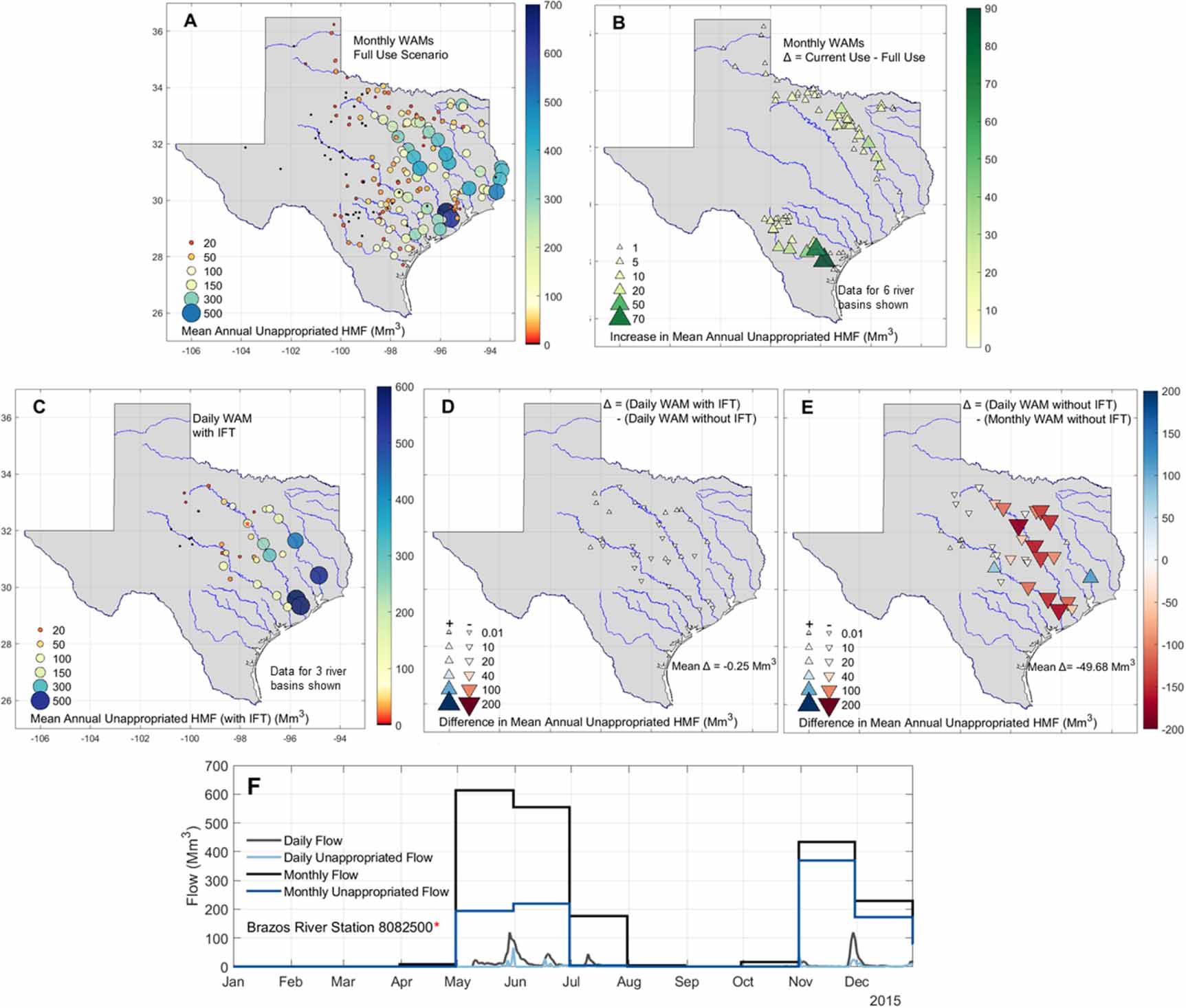
Figure 4. (a) Mean annual unappropriated HMFs estimated using the WAM full-use scenario. (b) Shows, for river basins with publicly available data, the increase in mean annual unappropriated HMFs when estimated with the WAM current-use scenario. Full-use assumes all allocated water is used by water rights holders and no return flows, and current-use is a best estimate of actual water usage including return flows. (c) Mean annual unappropriated HMF estimated with daily-timestep WAMs, including instream flow targets (IFT), showing spatial variation due to watershed climatology, water appropriations, and environmental factors. (d) Differences in mean annual unappropriated HMF with and without IFT, revealing minimal IFT impact. (e) Comparison between daily and monthly timestep WAMs (without IFT) showing a significant decrease in unappropriated HMF at the daily scale. (f) A time series from a Brazos River station (red asterisk in panel C) illustrates differences in total and unappropriated flows between daily and monthly timestep estimates.

Download figure:

Standard image High-resolution image

In contrast, the lowest magnitudes of unappropriated HMFs occurred in semi-arid west Texas, including the Canadian, Nueces, and Rio Grande river basins (figure 4(a), table S2). Although these stations have HMFs, flow magnitudes are low, and water rights allocations further limit the ‘availability’ of HMFs. Of the 190 stations, 28% (53) averaged < 10 Mm3 (∼0.008 maf) of unappropriated HMF/yr. Of these, 10% of the stations had no unappropriated HMFs for any years of record, primarily located in small watersheds in central and west Texas. The Colorado River, one of the major Texas rivers by flow, had nine stations (33% of the 27 total stations) with no unappropriated HMFs annually.

3.2.2. Unappropriated HMF using WAM current water use scenario

Averaged across all stations with data, the mean increase in annual unappropriated HMF in the current-use scenario with return flows was 10 Mm3 (∼0.01 maf) relative to the full-use scenario, a mean increase of 136% (figure 4(b); table S2). The difference in unappropriated flow between the current-use and full use provides insight into the unused or return flows that are already permitted by the TCEQ.

3.3. Unappropriated HMF and instream flow constraints estimated at daily timesteps

WAMs computed at daily timesteps were evaluated for the Brazos, Colorado, and Trinity River basins (figures 4(c)–(e)). These WAMs provide estimates of unappropriated flows at the daily level, allowing for estimation of unappropriated HMF, including IFT, at the timescale of storm events. Results are presented for daily WAM simulations both with and without IFT.

3.3.1. Including IFTs

Estimates of unappropriated HMFs from daily WAMs including IFT followed similar spatial trends to those of the monthly WAMs (figure 4(c)). However, the addition of IFTs had a minimal impact on HMF availability. This reduction in the volume of mean annual unappropriated HMF was <1%, with a mean magnitude of −0.25 Mm3 (200 af; figure 4(d), table S3) across all stations, with no clear spatial trend.

In a given year, the principal limiting factor on the volume of available HMF can be either a) the volume of HMF, b) water rights appropriations, and/or c) instream flow requirements. In the Brazos, Colorado, and Trinity river basins, low HMF volumes and water rights were the limiting factors for HMF availability in the upstream/low flow portions of the basins (figure 5; table S3).

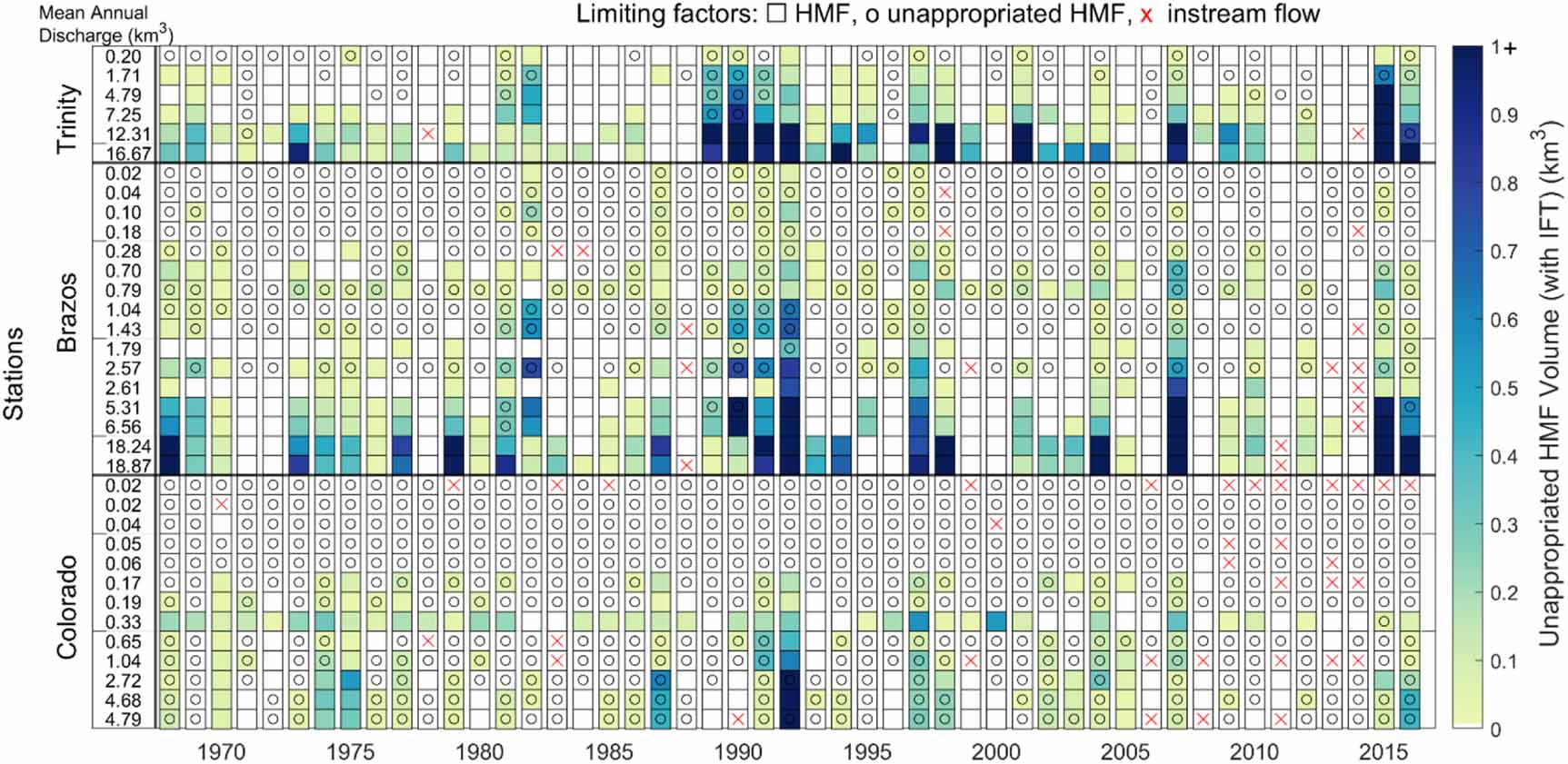
Figure 5. Total unappropriated HMF volumes depicted for the years 1968–2016 as estimated by the daily WAMs, including both water rights and instream flow requirements, where darker shades indicate higher unappropriated HMF volumes, exceeding 1 km3 (0.81 million acre-feet, maf) in the year. Stations in the three modeled river basins are sorted in descending order by their total discharge. Circles depict years in which water appropriations were the most common limiting factor for ‘available’ HMF, red x’s indicate environmental flows as the limiting factor, and no symbol indicates that the volume of storm flows were the limiting factor (table S5). Wet years, particularly those in the early 1990s, 2015, and 2016, commonly produced available HMF exceeding 1 km3 (0.81 maf). Between the wet years, however, stations with substantial available HMF were typically limited to the stations with the highest discharge in the relatively humid Brazos and Trinity River basins. Volumes of available HMF tends to scale with discharge at each station, and accordingly tend to increase with watershed size (i.e. further downstream or on the main stem of the river).

Download figure:

Standard image High-resolution image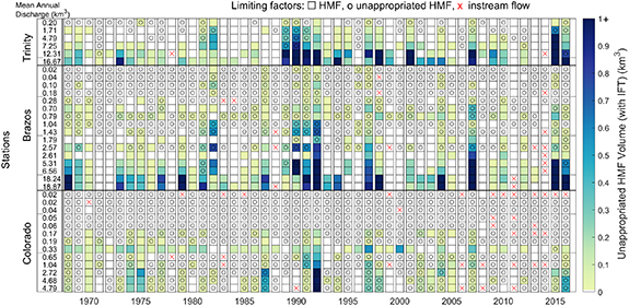

Instream flow requirements had a lower impact on HMF availability relative to water appropriations, but were still relevant in the three river basins. Instream flow requirements were most impactful during the dry period between 2008 and 2014, particularly in the Colorado River basin (figure 5). Being the most westward (and relatively arid) basin, the differences between prolonged dry periods and occasional wet years were most pronounced. For example, between 2008 and 2014 eight stations in the Colorado basin had no unappropriated HMFs for during that period (figure 5, table S3).

3.3.2. Comparison of unappropriated flows from monthly and daily WAMs

Estimating unappropriated HMF at a daily timestep, without including IFT, allows for direct comparison of unappropriated HMFs for daily and monthly WAMs. Mean annual unappropriated flows based on monthly WAMs exceeded those based on daily WAMs in 26 out of 35 stations by ∼50% in the Brazos, but were more variable in the Colorado and Trinity basins (table S3). Of these 26 stations, the average reduction in mean annual unappropriated HMFs was ∼0.07 km3 (0.06 maf; figure 5(e), table S3).

Across all 35 stations, mean annual unappropriated HMF was reduced by 36% (−49.68 Mm3, 0.04 maf) when using daily rather than monthly WAM estimates (table S3, figure 4(e)). All stations in the Brazos River basin, for example, had less mean annual unappropriated HMF in the daily WAM relative to the monthly WAM. HMF events occurred on a shorter timescale (days) than the aggregated monthly estimates of unappropriated flows, reducing the volume of unappropriated HMFs (figure 4(f)). Further, daily timestep WAMs include flood control operations for reservoirs in which storage in flood pools can limit flow magnitudes during large precipitation events [59].

3.4. Consideration of coastal inflow requirements

In addition to water rights and IFT, the potential for availability of HMFs also depends on compliance with coastal inflow requirements for rivers that drain into the sea. The prescribed flow regimes differ across river basins and and can range from static minimum monthly and annual required flows, seasonal minima that are modified by the hydrologic regime of a given year (i.e. drought years, wet years, normal years) and varying definitions for each season as stated in 30 TAC §298. The TCEQ adjudicates these additional requirements separately from the WAMs during the permitting process.

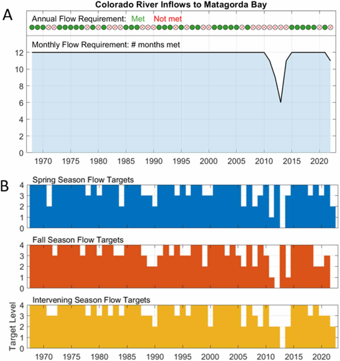
Coastal inflow requirements for the Colorado River, for example, were evaluated here using the furthest downstream USGS gage for 1968–2022 (figure 6). The annual threshold of 1.4 maf (1.7 km3) was met in 56% of years during this time period, below the target attainment frequency of 60%. This constrains the amount of new water permits that can be considered on the Colorado River. The adjudication of these coastal inflow requirements by the TCEQ sets further limitations on the quantity of HMFs that could be considered ‘available’. Additional tables and figures on coastal inflow standards for the Brazos, Colorado, and Trinity river basins are provided in supplemental information (Tables S9-S11; SI Section 4.2.2).

Figure 6. Time series showing the achievement of the annual inflow standards for the Colorado River into Matagorda bay (a) and the number of months per year in which the inflows met the monthly requirement (b). In the 55 year record in this analysis, the required annual inflow total of 1400 000 acre-feet (1.4 million acre-feet, maf) was met for 31 years, or 56% of the record. The monthly inflow requirement of 15 000 acre-feet (18.5 Mm3) was met 98% of the months (648 out of the total 660 months of record). Seasonal inflow targets, based on ‘levels’ of ecological health, were met to at least the minimum level in 54 of the 55 years of record (98%) in this study. The attainment frequencies with the seasonal inflow targets at all ecological levels exceeded the target frequency threshold (table S11).

Download figure:

Standard image High-resolution image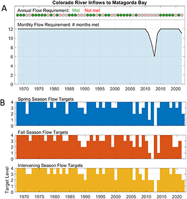

3.5. Accounting for the components of total streamflow

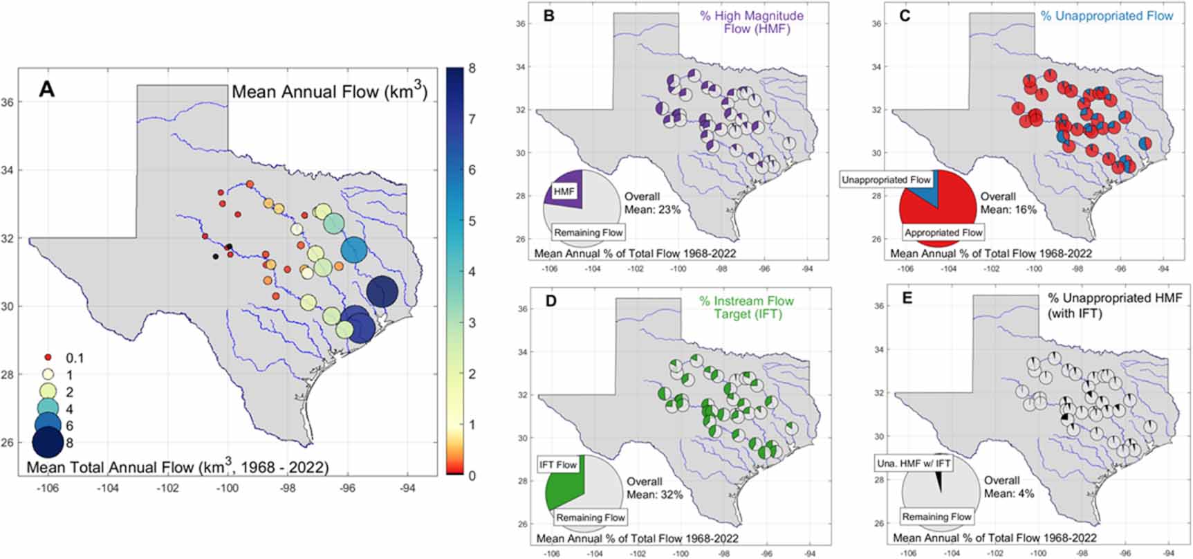
Using daily-scale WAM estimates, unappropriated flow (i.e. flow not reserved by water rights), HMFs, IFTs, and HMFs considering both water rights and IFTs were estimated (i.e. ‘available’ at that level). Of the stations located in the Brazos, Colorado, and Trinity river basins, the highest mean proportion of the total flow magnitude was HMF (33%, meaning one-third of total flow was from HMF events), followed by unappropriated flow (22%), IFT (20%), and unappropriated HMF with IFT (8%; figure 7, table S4). The small difference between unappropriated flow and IFT (mean 2%) reflects the fact that water appropriations in downstream stations typically reserve enough water to satisfy IFT (figures 5 and 6). The lowest percentages of unappropriated flows (relative to total flows) were associated with the highest percentages of HMFs, located in upstream stations in relatively small, semi-arid watersheds.

Figure 7. Percentages of the mean total annual flow of each station (a), split by its component parts including unappropriated flow (b), HMF (c), IFT (d), and unappropriated HMF (with IFT; (e) (table S4). Upstream stations had relatively low streamflows (a), with relatively higher proportions of HMF constituting their total flow (b). The proportion of unappropriated flows was generally lowest in the Colorado basin (mean 10% across all stations in the basin), followed by the Brazos (18%) and the Trinity (24%) basins (c). Similarly, the IFT as a percent of the total flow was highest in the Colorado basin (47%), the most arid of the three, followed by the Brazos (27%) and Trinity (17%) basins (d); Table S4). Combined, these limitations on ‘availability’ reduces the percentage of total flow that is unappropriated HMF also considering IFT (e).

Download figure:

Standard image High-resolution image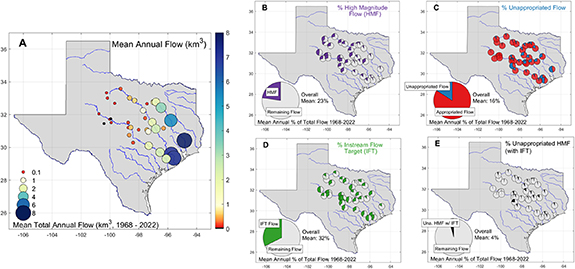

4.1. Addressing spatiotemporal disconnects in unappropriated HMFs

The distribution of HMFs, including unappropriated HMFs, is highly variable year to year and across different climatic regions within the context of demand and urban growth (figures 3 and 4). Results showed that HMFs depend strongly on climate and watershed size. The highest annual HMF totals, including HMFs considering water rights and instream flows, occurred in the humid southeast, or along the main stem of the major rivers. This creates disconnects between where and when water is available and where water is needed. Conveyance of water from areas of supply (rivers, reservoirs) to areas where MAR can be implemented can address the spatial disconnect, while banking of water for long-term storage with MAR addresses the temporal disconnect.

For HMFs to be feasibly used as a source for MAR, HMF availability needs to be collocated with water demand (which is driven by municipal, industrial, and/or agricultural needs). Statewide water demand has increased steadily over time and remains fairly consistent year-to-year (figure S14), but regional demand trends vary across the state [48]. In areas with high demand, the frequency and volume of available (permittable) HMFs, considering all constraints, should be sufficient to support the necessary infrastructure to support MAR.

Understanding future water demands is critical for guiding future implementation of HMFs for MAR. In Texas, annual water needs (potential shortages) are projected to reach 3.76 km3 (3.0 maf) for irrigation use and 3.88 km3 (3.1 maf) for municipal use by 2070 [48], making up 90% of the total water shortage (table S14). The highest usage of water for irrigation occurs in the High Plains region (northwest Texas) and the lower Rio Grande Valley (south Texas), whereas the highest municipal water usage occurs in urban areas. The use of HMFs for MAR may not be feasible for irrigation shortages, but may instead be most impactful for municipal water shortages where HMFs are more substantial.

These sub-regions provide context for MAR strategies that could be applied to areas beyond Texas with similar climate regimes and water scarcity concerns, such as the western US and Australia. Given variations in water demand, HMF availability, and hydrogeologic conditions, there is no single template by which MAR can be implemented at large scales using HMFs. Feasibility instead depends on site-specific characteristics including water rights, environmental flow requirements, conveyance of water, and the local storm climate [25, 60, 61]. Thus, the importance of local context for each project provides a challenge for upscaling these operations.

4.2. Optimal conjunctive use of water infrastructure for MAR

For HMFs to be a practical source for MAR, temporary storage of captured HMFs needs to be considered. This stems from the difference in timescales between high HMF rates and generally low infiltration/injection rates of MAR operations. Interim storage of captured HMFs is often required to address this disparity in flow rates [62]. To address this, conjunctive use of existing surface water reservoirs and MAR have been used to optimize water storage. Retrofitting urban HMF infrastructure for MAR has been used to passively promote recharge [62–64]. In Arizona, for example, this was achieved by adding dry wells or infiltration trenches to the low points of existing HMF detention and retention ponds so that sediment settling and biofiltration could treat HMF that was captured by the structures before infiltration [62].

Existing reservoir infrastructure has also been utilized to couple excess surface water and groundwater resources in both Texas [63] and California [65]. Agricultural MAR, widely implemented in California, addresses the interim storage problem by routing reservoir releases to agricultural fields to promote infiltration [16, 22]. This technique adds a secondary use for existing infrastructure, using existing reservoirs and active farmlands to minimize impact [66]. The city of Corpus Christi, Texas, utilizes the large storage capacity of nearby surface reservoirs to provide a source for ASR and reduce evapotranspiration [63]. In this case, MAR implementation is not limited by interim storage capacity, but instead by the number of wells feasible for injection. With increasing interest in the optimization of reservoir storage and operations [16, 26, 67, 68], conjunctive use of existing reservoirs and MAR could produce practical volumes of water capture and storage.

4.3. Legal limitations on availability of flows

The volume of water physically present in a water body is not indicative of the amount of water ‘available’ for capture. Surface water can only be used for MAR after proper permitting by the appropriate legal bodies, which in this study is the TCEQ. There are many complexities in the water permitting process, particularly with the alteration of existing permits and the granting of new permits [69]. Though extreme flow events produce ample volumes of water with respect to water needs (figure S14), only a certain fraction of that water may be considered permittable for use. This limitation inclu