1748-9326/20/11/114082

Abstract

International efforts to combat climate change almost inevitably entail relative earnings reductions for fossil fuel companies, and gains by renewable companies. This study investigates the relationship between climate change conference of the parties (COP) meetings and the stock market performance of selected publicly listed companies. Specifically, we compare the price formation of fossil fuel companies, ethically-rated (‘green’) companies and renewable energy companies during international climate negotiations, compared to the periods around them. We investigate changes in market behaviour during COPs using two different statistical approaches to assess both whole of the period and daily effects. Both methods find distinct increases in the values of stocks with high green ratings, but no changes in stocks of renewable companies and weaker and more statistically inconsistent decreases in the values of fossil fuel companies. No consistent results are found for variability measurements, other than general market variability increases during COPs. We show that, by contrast, Organization of the Petroleum Exporting Countries meetings produce very strong increases in the stock values and variabilities of fossil fuel companies, and fairly strong decreases in the value of renewables companies, showing that detectable changes during predictable events are generally plausible. We conclude that market behaviour so far appears to favour companies with lower environmental impact during COPs but does not convincingly shift company price formation in line with the necessary green transition.

Export citation and abstractBibTeXRIS

Since 1995, countries who are party to the UN Framework Convention on Climate Change have met at yearly climate meetings called conferences of the parties or ‘COPs’ (UNFCCC 1992). At these meetings, parties negotiate agreements aimed at limiting the impact of climate change through factors like emissions reduction pledges and promises of financial and technological transfers for climate mitigation or adaptation. The temperature goals stated in various agreements imply a strong reduction in the use of fossil fuels and an increase in renewable energy sources. Notably, the Glasgow Climate Pact, emerging from COP26 held in Glasgow in 2021, marked a significant departure by being the first COP agreement to explicitly include text on fossil fuels (UNFCCC 2021). This comes with the growing recognition of the need to address fossil fuel consumption directly in international climate conferences. If these developments are taken seriously by the market, we would expect to see changes in the valuation of the stock prices of relevant companies.

Previous studies have shown that stock markets respond to news of upcoming climate policies and legislation (Ramiah et al 2013, Birindelli and Chiappini 2021, Antoniuk and Leirvik 2024) or climate concerns of the traders or public (Alekseev et al 2022, Ardia et al 2023, Schuster et al 2023). This includes news relating to the Paris Agreement (COP21) (Pham et al 2019, Monasterolo and de Angelis 2020) and COP26 (Birindelli et al 2023, Pandey et al 2023, Ge et al 2024). Generally, these studies show that news about climate change increases the value of low-carbon companies and decreases that of carbon-intensive companies. However, typically, this literature has been very company- and/or country-specific and does not examine market response for fossil fuel companies more broadly. We address this gap here, noting that climate change mitigation scenarios produced by integrated assessment models suggest that limiting emissions enough to avoid even 2 °C of warming from pre-industrial temperatures by 2100—the limit of the 2010 Cancun agreement (COP16), and violating the ‘well below 2 °C’ limit of the Paris Agreement—would likely require substantial reductions in global fossil fuel use (Byers et al 2022, IPCC 2022, Kikstra et al 2022).

What does transition require? The possibility of carbon dioxide removal technologies or fossil fuel use with carbon capture and storage (CCS) means that we cannot translate a remaining carbon budget directly into an allowed fossil fuel quota (Bataille et al 2025). However, the expense of capturing carbon means consumption is still greatly curtailed. For instance, the capital cost of a coal or gas electricity generation facility with CCS is almost double that of one without CCS (Clarke et al 2022). In 99% of scenarios in the AR6 WGIII Scenarios database that keep warming below 2 °C this century, consumption of fossil fuels is projected to decrease between 2020 and 2050, with a median decrease of 44%. The median fossil fuel consumption increases for scenarios not limiting temperature rises below 2 °C by 10%. By contrast, renewable energy generation triples in the median <2 °C world scenarios, but only doubles in the median >2 °C world. This shows a huge difference in the future profitability of fossil fuel and renewable industries depending on climate action, hence we expect clear signals of future climate legislation should result in strong stock price effects. We pose several possible hypotheses:

1.

Climate success hypothesis: If COPs consistently raise climate ambition, we would expect the stock prices of renewable companies to rise and fossil fuel/carbon-intensive companies to fall relative to the expected behaviour during this period. There is some evidence that generic climate news stories from COPs could have this effect too (Engle et al 2020, Ardia et al 2023, Ma et al 2024).

2.

Market volatility hypothesis: If COPs inconsistently modify climate ambition, we would expect stock prices of these relevant companies to vary more during this time than during control periods. There need not be consistent climate action, but merely information on the level of climate action expected, for this effect to exist.

3.

Policy inefficacy hypothesis: If most COPs do not reveal information about global action but merely move money or emissions around, we would expect to see no reaction.

4.

ESG (environmental, social and governance) premium hypothesis: If markets only interpret the impacts of COPs through the frameworks of ESG metrics, then companies with green ratings will be advantaged, irrespective of the transition risk to the companies.

It may be argued that, as the schedules of these conferences are generally known well in advance and the results of them could often be anticipated, we should not expect them to result in a consistent shift as implied by the climate success hypothesis or the ESG premium hypothesis. We support the claim that such violations of the efficient market hypothesis are plausible by carrying out a similar analysis on Organization of the Petroleum Exporting Countries (OPEC) meetings, which are more frequent but shorter and therefore trends on them are subject to less statistical noise from correlated deviations.

When considering the ESG premium hypothesis, it is a well-recognised problem that different ratings systems diverge. This divergence in the ESG ratings across providers is well documented in the literature (Gibson Brandon et al 2021, Berg et al 2022, Christensen et al 2022). These studies highlight the discrepancies in how the different agencies assess ESGs. For instance, (Gibson Brandon et al 2021) demonstrate that pairwise correlations between ESG ratings from different providers are surprisingly low, a finding we replicate in the SI. The reason for the discrepancy is debated; (Berg et al 2022) find that measurement differences account for the largest portion of ESG rating divergence, followed by the scope of attributes used. Meanwhile, (Capizzi et al 2021) find that the social and governance components of the ESG are more relevant for explaining divergence in Italy, whereas (Christensen et al 2022) find more disagreement arising from rating outcome metrics.

We investigate the market movement in stocks during the period of COPs compared to other periods. In order to distinguish robust shifts from random noise, we consider two approaches. First, we compare differences in distributions of various properties of stock price during the approximate 2 week COPs relative to control periods of identical length without a COP directly preceding or following (what we term ‘pseudo-COPs’). Second, we apply a linear regression analysis with company-year fixed effects to examine daily changes.

2.1. Data collection and cleaning

For both statistical approaches, we focus on the largest publicly traded companies by market capitalisation to reduce variability. We select the 32 largest companies in each category that was publicly listed from at least the start of 2011 and passed data cleaning protocols, as rated by CompanysMarketCap.com. We chose 32 because it represented the complete set of renewable energy stocks meeting these criteria when the study was initiated, though we also consider the top 20 companies in each category (and top 100 fossil fuel companies) to investigate the robustness of results. While there are many older fossil fuel companies, the majority of the largest renewables companies do not date back to 2010. Daily stock price data are collected from Yahoo finance, and sustainability ratings are collected from sustainalytics.com. We categorise rated stocks based on their Sustainalytics rating, Neutral being medium risk, i.e. a 20–30 rating, Green being anything lower and high-impact being anything higher. This last category is mostly fossil fuel companies. Data is collected between 1 January 1990 and 25 February 2025 where market data is available. Companies are represented in most of the largest stock markets around the world, and though around half the companies are headquartered in the USA, they are generally multinationals with widespread legal exposure.

We note that the use of ESG ratings from Sustainalytics to categorise companies is one specific approach. Using ESG ratings from a different rating agency, S&P, yields similar overall trends but with notable numerical differences, as detailed in the SI. Generally S&P gives better rankings to fossil fuel companies, and is therefore not our first choice of ESG metric.

Data cleaning is performed in two stages to reflect the different analytical approaches. The first stage applies to all data and addresses periods of market inactivity. Stocks with over 40 consecutive market days (days when the market is open) with 0 trading and 0 change in value after 2010 are excluded. Stocks are also removed if they exhibit such inactivity periods at any time, combined with the stock close price either doubling or halving between sequential trading days. Otherwise, the data before the period of nontrading and the 50 calendar days after it are removed to avoid the influence of protracted post-disruption volatility.

The second stage applies stricter criteria specifically for the daily linear regression analysis. This stage excludes days on which there are stock splits; daily changes of more than 50% to the value of the stock; days with negative close prices; and market days which either have or are next to a market day that had a market volume below 100. These additional cleaning steps mean that the daily linear approach is cleaner and more sensitive to smaller changes, but potentially biased against big changes that might be linked to COP events. Finally, we should note that the whole period method does not account for the non-trading days in the control period.

2.2. Whole of period analysis (COPs vs. Pseudo-COPs)

We firstly investigate how the stock price changed during the whole period of each COP (usually around two weeks long, although in some cases as short as 9 d) compared to the same period moved forwards or backwards by an even integer number of weeks, between −24 and +24, resulting in a total of 25 examined periods (12 before + COP period + 12 after). We refer to the periods with nonzero weekly shift as pseudo-COPs. This descriptive comparison reveals whether changes during COP events differ statistically from periods without COP events. To prevent contamination, we exclude pseudo-COPs starting within 3 weeks of the actual start of COP from the analysis, as these may incorporate delayed or anticipatory effects, or overlap with the actual COP.

Our statistical approach assumes that stock price movement is best treated as a fraction of the current value, as is appropriate for stocks that approximate geometric Brownian motion (Mantegna and Stanley 1999, Cont 2001). We therefore investigate the proportional change in value between close-of-market values the day before the period starts and the day after it ends. This method accounts for large price fluctuations over time.

We also investigate the stock price volatility during each period. To do so, we calculate the geometric standard deviation (i.e. standard deviation in log space, gSD) in the daily close price across the period compared to the control group. Stock prices may change by an order of magnitude across the time period investigated, and loosely conform to a geometric random walk (Sabir and Santhanam 2014), so the gSD is more appropriate than the standard deviation in linear space. We normalise the gSD of each company to 1 across the whole time period before averaging and comparing them, to ensure that the volatility measures are comparable regardless of the companies’ stock volatility.

For each portfolio (neutral rated, green rated, fossil and renewable) we compare both the proportional price changes and gSD changes between COP and pseudo-COP periods. We also perform the same analysis for OPEC meetings for comparison. We subtract the changes in the neutral 32 portfolio during each time in order to control for market-wide movements, and hence better identify changes during COP.

Finally, we rank the actual COP amongst the set of pseudo-COPs, in terms of price change and volatility. This fractional ranking can be converted to a cumulative probability of having a rank this extreme via the relationship in (Folland and Anderson 2002) to assess the evidence of statistically significant difference in stock price during COP events, relative to pseudo-COPs. If the COP’s rank is very high or very low compared to the pseudo-COPs, it suggests a significant shift.

2.3. Daily linear regression analysis

We also implement a daily linear regression analysis with company-year fixed effects to examine the difference in daily stock price fluctuations during COP events, relative to other periods, controlling for various factors. The idea is to express the daily fractional changes in stock price as linear combinations of several components shown in equation (1)

where is the coefficient corresponding to the average market movement , the average fractional change in a neutral portfolio (usually the 32 neutral-rated companies, though we also consider the results using the S&P 500 in the SI). captures company-year fixed effects, to control for the company’s characteristics within a given year and any level differences across years for that company. is 1 when the year of time t is y and 0 otherwise is the coefficient corresponding to the Risk-free interest rate effect (), incorporated using a 13 week treasury bill (ticker ^IRX), interpolated for days when the USA market is closed. This is important to reflect the fact that the rate of return in riskier assets is often compared to that of safer assets, and so changes in this rate can affect different sectors differently (Krishnamurthy and Vissing-Jorgensen 2012, Gorton and Ordoñez 2022). is the coefficient of interest, determining the effect of the COP period indicator, , a dummy variable equalling 1 if the time is within a COP meeting and 0 otherwise. The error term captures the unexplained variation.

We use an ordinary least squares estimator from the python pyfixest library package to estimate the parameters of this linear regression model. This is a python implementation of the R package fixest, based on (Bergé 2018). We use a measure of errors clustered at each company level. In the supplementary information (SI) we show results from repeating the same exercise using a different python package (sklearn), with no error clustering. We also apply the same model to estimate the daily range of values of a stock price (the difference between the highest and lowest values) as a fraction of the highest stock price, a measure of the daily variability. We perform robustness checks here by running equation (1) without the risk-free rate term, and derive very similar results in the SI.

We also examine a modification of equation (1) where we add a coefficient for each specific COP time. This allows us to see if stock price variations during COP events change systematically across time as we obtain an estimate of the coefficient for each specific COP event. This is shown in equation (2):

where we have added the term to represent the number of the COP itself (0 in the first year, 1995, and set to −1 for times outside of COPs) and solve for the new coefficient of interest as well.

Finally, we conduct a similar analysis for OPEC meetings. Only the daily linear regression analysis with company-year fixed effects is directly applicable, given that these meetings tend to last for 1 day.

We estimate these linear regression models using the full panel dataset, described in SI table S1, which includes an overview of the number of companies and observations.

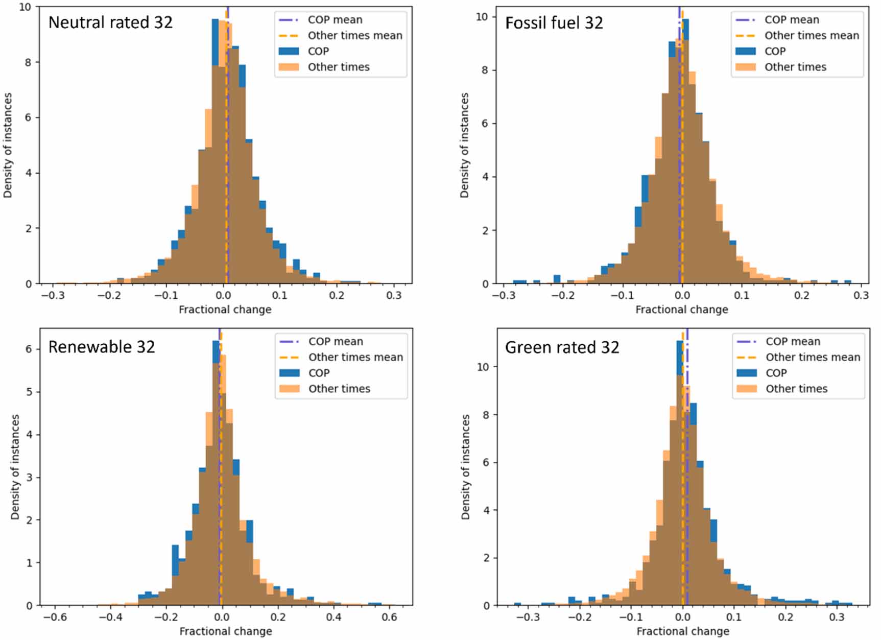
Table 1 shows the results of this analysis. Interestingly the daily model indicates that the COP periods have an anomalous effect on the daily range of values seen, though this is not seen in the standard deviation of closing prices throughout the week. The differences in these two measures of volatility suggest that there may be some market response to news coming from COPs, but it tends to wash out rapidly. A two-sided test for the whole-period comparison will never return below a 5% probability—there are only 22 neutral fortnights in the year and the conversion of ranks into probabilities imposes an additional uncertainty. However the fact that the period with the most extreme result occurs during COP for the top 20 green companies is a strong indication that this period is anomalous. This result is substantiated in figure 1, where there is a distinct preponderance of higher fractional change periods during COPs for green-rated companies, but smaller differences for other distributions.

Figure 1. Proportional change in stock prices for different portfolios during the period of each COP, or similar time periods shifted by between 3 and 24 weeks. All portfolios except the neutral portfolio have the neutral portfolio’s trend subtracted from them. Events more than 5 standard deviations from the mean of all data are removed for clarity.

Download figure:

Standard image High-resolution image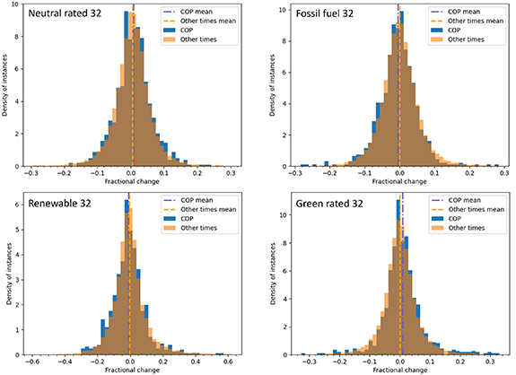

Table 1. Differences between COP and non-COP periods. The whole period method compares the period of COPs to a shift of the same period by some weeks. Rank results indicate how the average proportional price change or variability during COP compares to the same statistics during pseudo-COPs. Note these results are naturally quantised and that the p value for the two-tailed tests for extremeness cannot be under 0.05 for the whole period comparison. The linear model investigates the changes during the course of each single day during the COP, compared to normal daily changes. The reported value is in equation (1), plus or minus one standard error. Probabilities (p) are also quoted, values below 0.05 are starred and values below 0.01 are double-starred. The neutral rated groups do not have a control group to subtract, the other groups use the neutral 32 results as their baseline.

| | Whole period comparison | Daily linear model | Portfolio | Diff rank | Diff p | gSD rank | gSD p | COP diff term | COP diff p | COP range term | COP range p | | | ———————– | —————— | ——— | ——— | –––– | –––– | —–– | ———–– | ———— | ––––––– | ———–– | | Neutral rated 20 (no control) | 0.652 | 0.743 | 0.348 | 0.658 | 0.0002 ± 0.0002 | 0.3825 | 0.0005 ± 0.0002 | 0.0061** | | Neutral rated 32 (no control) | 0.739 | 0.572 | 0.478 | 0.914 | 0.0002 ± 0.0002 | 0.3364 | 0.0005 ± 0.0001 | 0.0012** | | Green rated 20 | 1.00 | 0.059 | 0.957 | 0.145 | 0.0013 ± 0.0004 | 0.0058** | 0.0003 ± 0.0003 | 0.3692 | | Green rated 32 | 1.00 | 0.059 | 0.957 | 0.145 | 0.0009 ± 0.0003 | 0.0035** | 0.0003 ± 0.0002 | 0.1879 | | Fossil 20 | 0.261 | 0.487 | 0.826 | 0.401 | −0.0005 ± 0.0002 | 0.0169* | 0.0000 ± 0.0002 | 0.8574 | | Fossil 32 | 0.261 | 0.487 | 0.87 | 0.316 | −0.0004 ± 0.0002 | 0.0460* | 0.0001 ± 0.0002 | 0.7834 | | Renewable 20 | 0.304 | 0.572 | 0.696 | 0.658 | −0.0006 ± 0.0005 | 0.226 | 0.0009 ± 0.0005 | 0.0609 | | Renewable 32 | 0.043 | 0.059 | 0.696 | 0.658 | −0.0006 ± 0.0004 | 0.1378 | 0.0009 ± 0.0005 | 0.0715 |

The daily model supports the claim that green portfolios experience unusually large value growth during COPs, with very small p-values for the green portfolios of both sizes. Weaker results (approximately half the size) are found in the daily model indicating a reduction in the value of fossil fuel companies, with no strong confirmation of this effect in the whole period comparison. The distributions behind this result are visualised in figure 2.

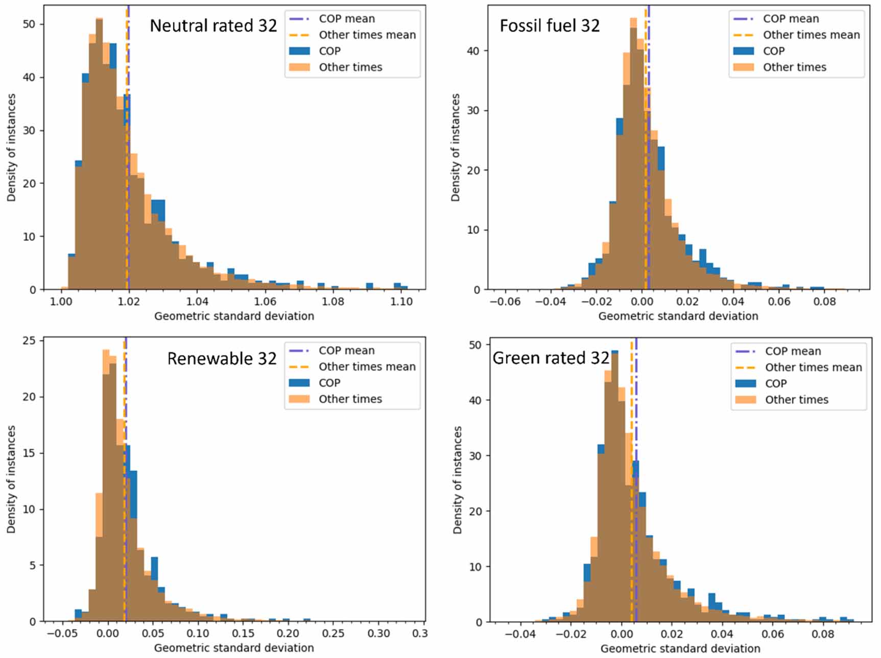
Figure 2. Plots of the geometric standard deviation (gSD) of different portfolios, either during COPs or during periods of the same duration between 3 and 24 weeks before and after. Events where the gSD varied from the average by more than 5 times the standard deviation of all gSD data are removed for clarity. All portfolios except the neutral portfolio have the neutral portfolio’s trend subtracted from them.

Download figure:

Standard image High-resolution image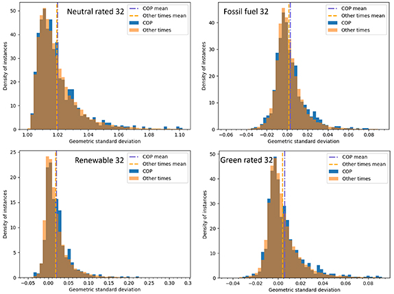

This green portfolio result is very robust. In the SI we report several alternative specifications of the model—leaving out the interest rate term in table S2, using an alternative linear fitting algorithm with different standard errors in table S3, and in table S4 using the S&P 500 index is used as the neutral group. By contrast, the other significant result in this table, that fossil fuel companies experience a decrease in valuation, is not robust under a change in the fitting algorithm, as well as not being found in the whole period method. In some alternative specifications, specifically the alternative fitting algorithm and using the S&P 500 as the neutral group, there is a significant effect for COPs increasing the range of values seen by renewables. There are also inconsistent signs of an increase in the variability of green-rated firms. Otherwise the various specifications of the models are in agreement that nothing noteworthy is happening.

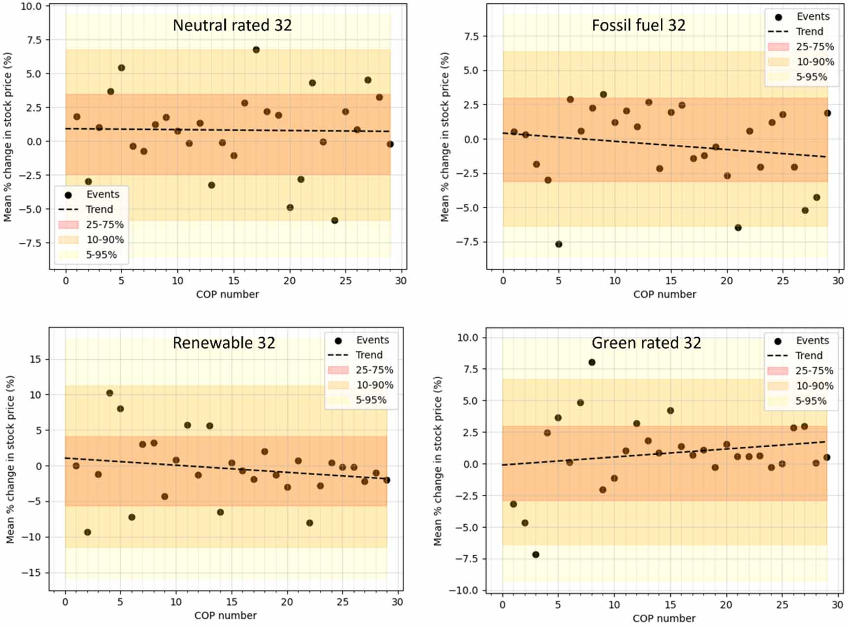
Table 2 shows that the neutral-rated stocks exhibit no significant long-term change during COPs (given that the confidence interval is spanning around zero). This is substantiated in figure 3, which also shows no trend in this. There is an inconsistent sign of an increase in their variability. There are stronger signs that the performance of fossil fuel companies during COPs is getting significantly worse with time, according to the daily linear model, though this is not robustly seen in the whole-period comparison. There are also signs of a similar downwards performance trend for renewable companies, and this result is robust across both statistical approaches.

Figure 3. Plots of the mean change in stock prices of sets of stocks across different numbered COPs. Background colouring indicates quantiles of stock price change across pseudo-COP periods. Dashed lines represent best fits to these.

Download figure:

Standard image High-resolution image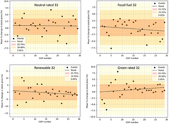

Table 2. How responses to COPs are changing with time. Whole period comparisons present the best estimate and the [5%–95%] confidence interval on the gradient of trend lines between COP number and the mean of either the fractional change or gSD of stocks in a portfolio. Daily linear model columns denote the coefficient of the COP number term , with the p-value of getting a value this large by chance in brackets. Probabilities below 0.05 are starred.

| | Whole period comparison | Daily linear model | Portfolio | COP period trend diff fit | COP period trend gSD fit | COP trend linear diff term × 1000 | COP trend p | COP trend linear range term × 1000 | COP range p | | | ———————– | —————— | ——— | ———————–– | ———————— | ––––––––––––––––– | ———–– | ———————————– | ———–– | | Neutral rated 20 | −0.0076 (−0.1358–0.1206) | −0.0076 (−0.1358–0.1206) | −0.0009 ± 0.0140 | 0.9489 | (0.0426 ± 0.0286) | 0.1538 | | Neutral rated 32 | −0.0068 (−0.1425–0.1289) | −0.0068 (−0.1425–0.1289) | 0.0081 ± 0.0155 | 0.6034 | (0.0362 ± 0.0235) | 0.1342 | | Green rated 20 | 0.0446 (−0.1401–0.2293) | 0.0446 (−0.1401–0.2293) | 0.0100 ± 0.0366 | 0.7872 | (−0.0362 ± 0.0290) | 0.2271 | | Green rated 32 | 0.0633 (−0.0682–0.1948) | 0.0633 (−0.0682–0.1948) | 0.0526 ± 0.0298 | 0.0879 | (−0.0303 ± 0.0198) | 0.1373 | | Fossil 20 | −0.0608 (−0.1855–0.0638) | −0.0608 (−0.1855–0.0638) | −0.0826 ± 0.0291 | 0.0105* | (−0.0474 ± 0.0224) | 0.0479* | | Fossil 32 | −0.0598 (−0.1913–0.0717) | −0.0598 (−0.1913–0.0717) | −0.0727 ± 0.0245 | 0.0056** | (−0.0238 ± 0.0213) | 0.273 | | Renewable 20 | −0.1736 (−0.3280—− 0.0192) | −0.1736 (−0.3280—− 0.0192) | −0.2032 ± 0.0531 | 0.0011** | (0.1485 ± 0.0685) | 0.0431* | | Renewable 32 | −0.1002 (−0.3030–0.1025) | −0.1002 (−0.3030–0.1025) | −0.1340 ± 0.0482 | 0.0092** | (0.2917 ± 0.0756) | 0.0005** |

Applying the same methodology to OPEC meetings gives the results in table 3. These show that OPEC meetings coincide with substantial increases in the value of fossil fuel company stocks, and in their variability, with both effects well below 5% probability. They also coincide with improved performances of neutral stocks, though with less statistical confidence. The strength of the changes in fossil fuel company valuation is around double that seen in for green-rated companies during COPs.

Table 3. Differences between stock performance during OPEC meetings compared to non-OPEC meetings, using the daily linear model. Probabilities below 0.05 are starred and those below 0.01 are double-starred.

Portfolio	OPEC diff	OPEC diff p-val	OPEC range	OPEC range p-val
Neutral rated 20 (no control)	−0.0004 ± 0.0003	0.2025	0.0003 ± 0.0002	0.2168
Neutral rated 32 (no control)	−0.0002 ± 0.0002	0.4888	0.0004 ± 0.0002	0.0465*
Green rated 20	−0.0004 ± 0.0004	0.2563	0.0002 ± 0.0003	0.4516
Green rated 32	−0.0001 ± 0.0003	0.7004	0.0002 ± 0.0002	0.1859
Fossil 20	0.0025 ± 0.0005	0.0001**	0.0013 ± 0.0003	0.0010**
Fossil 32	0.0025 ± 0.0004	0.0000**	0.0011 ± 0.0003	0.0005**
Renewable 20	−0.0020 ± 0.0006	0.0029**	0.0015 ± 0.0005	0.0100*
Renewable 32	−0.0012 ± 0.0006	0.0539	0.0017 ± 0.0005	0.0044**

On one level these fossil fuel company effects are unsurprising, given that OPEC meetings often result in increasing or stabilising global oil prices, increasing the value of fossil fuel companies. On another level, this appears to be a market failure as net market movement effect could clearly have been anticipated in advance. Overall, the results indicate that OPEC meetings coincide with a considerably stronger and more consistent daily market change than during COPs, especially on fossil fuel company stocks.

Given the increasing prominence of climate policy and the potential for significant shifts in the energy sector, understanding how international climate conferences (COPs) affect financial markets is crucial. We investigate whether COPs are associated with a shift in stock market valuations of companies expected to be affected by the transition to a low-carbon economy, and show that some associations are detectable, meaning that COPs are taken seriously by stock markets, but that the strongest of these effects are more concerned with company ratings of greenness than the actual needs of a low-carbon economy. It is important to note that the ESG categorisation varies among rating agencies, and that alternative rating systems may not show any significant signs of this phenomenon. We also remark that these patterns are not guaranteed to persist into the future and should not be interpreted as investment advice.

Going through our four proposed hypotheses, our findings provide little support for the climate success hypothesis (hypothesis 1)—while there are effects that are not priced in, the strongest of these are not well-correlated with the requirements of transition. There are inconsistent and weak signs of reductions in the values of fossil fuel companies and in some model specifications, variability increases for renewables in the linear daily model, however these are not seen in the whole-period model. This means we also see little evidence for the market volatility hypothesis (hypothesis 2). We have evidence against the policy inefficacy hypothesis (hypothesis 3, that COPs are entirely ignored by markets), as some effects were robustly detected. But we have strong support for hypothesis 4, the ESG premium hypothesis. This indicates that news from COPs is received by the market, but most prominently channelled through the prism of ESG metrics rather than an actual need to transition away from fossil fuels or towards renewable energy. There are signals that more recent COPs are associated with more stock value losses for fossil fuel companies, however this is tempered by signs that they are also associated with worse performances for renewables companies too. The changing trend over time could explain why the whole-period detection methods do not indicate a notable COP penalty for fossil fuel companies, but the daily method, with a higher sample size to work with, does detect a statistical difference. Together this leads to our main conclusion that while price formation among companies with favourable ESG metrics appears to move with COP signals, the same is not evident for renewable energy companies more broadly.

Our analysis also highlights that OPEC meetings are associated with a more pronounced and consistent change the fossil fuel stock performance than COP meetings. This makes sense, due to OPEC’s role in reinforcing fossil fuel output and hence price stability. While the strength of the association may be due to the shorter duration of the meetings as much as the actual impacts, it shows there is a route to detectable market judgements on policies in the short term.

In terms of other limitations, our analysis focuses primarily on large-cap companies, and the results may not generalise to smaller companies. Furthermore, our analysis remains descriptive as isolating the causal impact of COP events from other concurrent economic and political factors is inherently challenging.

The findings nevertheless have important policy implications. If international climate conference aim to drive meaningful financial market shifts, they must move beyond broad commitments and provide clearer, binding policy signals that directly impact company valuations. This could include stronger commitments on fossil fuel phase-out, and more clarity on pricing mechanisms such as carbon markets. Future research could explore the mechanisms through which COP decisions might indirectly affect market dynamics and hence have implications for climate policy effectiveness. Future research directions could also explore whether specific COPs announcements have affected stock markets, as well as what news investors are looking for to allocate resources consistently with a low-carbon transition.

We thank Lakshmi Sannapureddy for useful comments when making this paper. Alaa Al Khourdajie was supported by the European Union’s Horizon Europe research and innovation programme under Grant Agreement No. 101056306 (IAM COMPACT) and Grant No. 101081179 (DIAMOND). Setu Pelz acknowledges funding from the European Union’s Horizon Europe Research and Innovation Programme under Grant Number 101056873 (ELEVATE).

The codebase required to perform this calculation is available at github https://github.com/Rlamboll/HowStocksJudgeCops and a frozen version of it uploaded to zenodo https://doi.org/10.5281/zenodo.17378710.

No conflicts of interest.

Data was publicly available from yahoo finance, Sustainalytics and S&P databases. OPEC dates were taken from their press release page. The code to automatically download the data from yahoo finance is part of the general codebase for the project, available from the github repository. The other data required is also uploaded to the github.

No ethical statement required.