1748-9326/20/11/114076

Abstract

Quantifying changes in loss of native vegetation cover relative to its coverage in protected areas (PAs) offers a valuable means of evaluating conservation performance, yet this approach is rarely applied in practice. Here, we assessed historic and recent remnant woody vegetation loss and protection across Queensland, Australia’s most biodiverse state. By comparing the proportion of remnant woody vegetation loss with the extent of formally PAs across 13 bioregions and 116 subregions, we generate a balanced evaluation of conservation progress and apply a risk classification framework. We found that Queensland has lost 21.4% of its original woody vegetation since European colonisation, with only 9.6% currently protected. Importantly, one-fifth of this loss occurred between 2000 and 2018, despite protection more than doubling during the same period. Our results show that protection gains were concentrated in low-risk regions, while areas with considerable historical loss, such as the Brigalow Belt and Mulga Lands, continued to experience clearing and low protection gains. By 2018, 44% of subregions fell into high or very high-risk categories, while only 15% were classified as not at risk. The risk status for most subregions remained unchanged, which suggests that limited conservation progress has been achieved in high-pressure landscapes. Our findings highlight the limitations of using protected area expansion alone as a metric of conservation progress. A balance-sheet approach tracking both protection and loss can provide a more robust framework for evaluating conservation outcomes. This type of balance-sheet framework can support more effective conservation planning, including restoration and stricter land-clearing controls. Our results offer practical insights for aligning national actions with global biodiversity targets, such as those outlined in the Kunming-Montreal Global Biodiversity Framework.

Export citation and abstractBibTeXRIS

The clearing of native vegetation causes habitat loss, fragmentation, and degradation, all major drivers of biodiversity decline worldwide (Maxwell et al 2016, IPBES 2019). Australia illustrates this global pattern (Legge et al 2023), having lost about 40% of its forests and between 47%–78% of its tidal marsh and mangrove extent since European colonisation (Bradshaw 2012, Serrano et al 2019). Losses have continued in recent decades, with over 7.7 million hectares of threatened species’ habitat cleared between 2000 and 2017 (Ward et al 2019), contributing to Australia´s high species extinction rate (Legge et al 2023, Woinarski et al 2024). Presently, over 2000 Australian taxa are listed as at risk of extinction, and 89% of ecosystems are showing signs of collapse (Bergstrom et al 2021). In response, policies oriented towards habitat retention and restoration are now widely recognised as critical conservation strategies (Ward et al 2021, CBD 2022, Kearney et al 2023), alongside the broader need to transform the social and economic systems driving biodiversity loss (SBTN 2020, DCCEEW 2022).

Protected areas (PAs) can reduce biodiversity loss within their boundaries (Joppa and Pfaff 2011, Geldmann et al 2013, Kearney et al 2020). Consequently, PA targets have gained prominence in major global conservation policies, including those set by the Convention on Biological Diversity (CBD 2010, 2022). This has led to an emphasis on expanding PA extent, and on reporting this growth as an indicator of conservation progress (McDonald-Madden et al 2009). However, while PAs can reduce biodiversity loss within their boundaries, they do not address threats outside them, nor guarantee long-term conservation (Pressey et al 2021). Indeed, species extinctions across Australia have occurred more commonly in bioregions with higher protected area coverage (Woinarski et al 2019), in part because PAs’ effectiveness at preventing loss is often limited by biases in their location, such as in less productive and remote lands (Hernandez et al 2021).

Assessments highlighting increases in PA coverage without accounting for concurrent biodiversity loss can create a misleading perception of conservation progress (Cook et al 2019). A more comprehensive approach is to balance biodiversity gains (e.g., PA expansion, improved representation) against concurrent losses (e.g., clearing, species decline) in a ‘conservation balance sheet’ (Hoekstra et al 2004, McDonald-Madden et al 2009, Watson et al 2016). Without this perspective, policy-makers cannot evaluate progress toward national and global biodiversity goals, such as protecting at least 30% of terrestrial ecosystems by 2030 (CBD 2022) and halting biodiversity loss through improved habitat retention and restoration (Commonwealth of Australia 2024). Yet reporting often focuses on gains or losses separately, rather than integrating them (Cook et al 2019).

In this study, we aim to illustrate the value of a ‘conservation balance sheet’ approach by jointly assessing remnant woody vegetation ‘gains’ (representation inside PAs) and losses (mainly due to land clearing inside and outside PAs). Using Queensland as a case study, we quantified historic losses since European colonisation and recent changes between 2000 and 2018, highlighting implications for conservation priorities. Remnant woody vegetation refers to native woody vegetation not cleared or substantially disturbed since European colonisation, excluding regrowth and non-woody types to ensure comparability with available datasets. ‘Conservation outcomes’ are measurable changes in remnant woody vegetation lost through clearing or secured within PAs. As a secondary aim, we use the gains-losses data to apply a risk classification framework that can provide insights for targeted policy and planning.

Queensland, Australia’s most biodiverse state, also has the country’s highest deforestation rate despite a mix of conservation strategies, such as PAs, the Environment Protection and Biodiversity Conservation Act 1999 (EPBC Act), the vegetation management framework (VMF), and restoration initiatives. However, Queensland has the nation’s lowest PA coverage, while the EPBC Act’s effectiveness is undermined by non-compliance, and that of the VMF by periodic amendments or exceptions (Hernandez et al 2024, Thomas et al 2025). Therefore, woody vegetation loss poses a significant threat to terrestrial habitat (Evans et al 2011, Neldner et al 2017, Queensland Government 2020), adopting Hall and colleagues’ (Hall et al 1997) definition of habitat as the resources and conditions that support occupancy, survival, and reproduction of organisms. Considering Queensland’s size (larger than most countries) these losses are globally significant (Pacheco et al 2021). If persistent clearing is not adequately addressed, expanding PAs will have limited benefits for most threatened species. Our study provides a comprehensive assessment of woody vegetation loss and protection over space and time, offering insights for conservation planning and identifying high-risk regions where targeted policy interventions are urgently needed.

To quantify historical and recent changes in remnant woody vegetation gains (coverage inside PAs) and losses (inside or outside PAs) across Queensland, we carried out spatial (overlay) analysis, using the data and processes described below. We then applied a risk classification framework to Queensland’s subregions. All data were processed in raster format (30 m) using ArcGIS Pro 3.0.3 and the Australia Albers equal area projection; complete data citations are listed in the supplementary materials.

2.1. Queensland’s bioregions and subregions

We assessed Queensland’s 13 bioregions and 116 nested subregions (figure 1(a)) to evaluate the representativeness of remnant woody vegetation in the protected area network and compare it with patterns of vegetation loss. In Australia, bioregions are geographically distinct landscapes defined by climate, ecological features, and species communities, and subregions further divide these landscapes based on finer-scale biophysical characteristics that influence species assemblages (Thackway and Cresswell 1995). Sixteen subregions with less than one-third woody cover in their pre-clearing extent were excluded. We used Queensland´s Biogeographic Bioregions and Subregions (Queensland Government 2010).

Figure 1. Queensland bioregions (a) gains (protection) and losses of remnant woody vegetation across time (expressed as a percentage of its extent (996077 km2) in 2000 (b). Gains (c) and losses (d) are represented spatially.

Download figure:

Standard image High-resolution image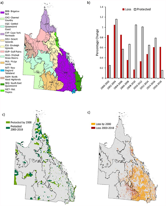

2.2. Quantifying remnant woody vegetation loss between 2000 and 2018 and mapping woody vegetation extent in 2000

We restricted our analysis to remnant woody vegetation due to the availability of high-quality clearing data produced since 1988 by Queensland’s Statewide Landcover and Trees Study (SLATS). SLATS monitors annual changes in the extent of woody vegetation due to human-induced land clearing, using satellite imagery and field data, initially using a probability model validated by image interpreters with high-resolution satellite sources (Queensland Department of Environment and Science 2022). Clearing events are also attributed to specific drivers. A small proportion of mapped loss corresponds to natural disturbances such as cyclones and tree mortality. These events accounted for less than 4.5% (2,345 km2) of statewide losses during 2000–2018 (77% occurring in the Wet Tropics bioregion) and were retained in our analysis to ensure consistent and comparable estimates of total woody-vegetation change across regions. We used SLATS 30 m raster data to quantify loss from 2000 to 2018. Although SLATS continues to map clearing, our analysis ends in 2018, as a change in methodology after this date limits comparability with earlier data (Queensland Department of Environment and Science 2022).

To quantify remnant woody vegetation loss within bioregions and subregions, we used Queensland’s 2018 woody vegetation extent map as a baseline and reconstructed change backwards (Queensland Government 2023). The 2018 dataset, derived from a neural network model based on very high-resolution imagery and manually validated (Flood et al 2019), was resampled from its original 10 m resolution to 30 m to match earlier SLATS data. We then added all pixels recorded as cleared between 2000 and 2017 in SLATS annual loss data, to the mapped woody vegetation in 2018. This approach enabled us to estimate loss between 2000 and 2018 and reconstruct remnant woody vegetation extent for the year 2000. It assumes that vegetation present in 2018 and cleared between 2000 and 2018 was also present and remnant at the start of 2000. By overlaying annual SLATS layers, we identified areas cleared in multiple years and determined the first year of clearing. We then summarised losses within bioregions and subregions to support regional comparisons.

We classified both fully and partially cleared vegetation in SLATS as loss. ‘Fully cleared’ refers to human-induced removal that reduces woody crown cover to below 10%, effectively converting the area to non-woody, whereas ‘partially cleared’ refers to clearing that affects more than 50% of woody vegetation, but where some vegetation remains (i.e. crown cover stays above 10%). Therefore, in this study, loss includes not only the complete removal of vegetation but also substantial degradation (including from natural disturbances). We do this because, once vegetation becomes highly degraded, it loses much of its ecological function (Watson et al 2018, López-Bedoya et al 2022) which is known to be highly detrimental to habitat-specialist species (Betts et al 2022, Filer et al 2022, Lindenmayer 2023).

2.3. Determining woody vegetation loss before 2000

To place recent changes in a historical context, we estimated loss prior to 2000 relative to a pre-clearing baseline. To this end, we overlaid Queensland’s 2000 remnant woody vegetation extent with a pre-clearing (pre-1750) Broad vegetation groups layer (Neldner et al 2023). Pre-1750 refers to the vegetation extent estimated to be present before European settlement and used here to represent a native woody vegetation baseline. To ensure compatibility with SLATS data, we excluded non-woody vegetation types by removing groups not classified as woodland or forest. This step allowed us to isolate cleared woody vegetation consistent with the SLATS loss data for 2000–2018.

2.4. Determining woody vegetation within PAs between 2000 and 2018

Protected area data were obtained from the Collaborative Australian Protected Areas Database (CAPAD) (Commonwealth of Australia 2023), compiled biennially by the Australian Government to report progress towards the CBD protected area targets. We included all designated terrestrial PAs, irrespective of IUCN management categories. While tracking gains and losses in other effective area-based conservation measures would be relevant as part of reporting towards 30 × 30 targets, they were not included here, as these are not yet comprehensively mapped in Queensland. To quantify changes in protection, we overlaid remnant woody vegetation layers with CAPAD boundaries at two-year intervals (2000–2018), when PA coverage increased from 4% to 8.7% of the state. This enabled us to quantify the extent of remnant woody vegetation within PAs at each time point. Vegetation lost after PA designation was excluded from protection counts and recorded as losses. Gains are defined as increases in remnant woody vegetation inside PAs; losses are clearing events inside and outside PAs, providing a conservation ‘balance sheet.’

2.5. Relationship between remnant woody vegetation protection and clearing

We assessed the threat risk of bioregions and subregions in 2000 and 2018 using a framework adapted from Hoekstra et al (2004) and Watson et al (2016). This framework uses the proportion of woody vegetation lost, protected, and an index that measures net positive change (F) relative to a pre-1750 baseline (McDonald-Madden et al 2009). F was calculated, for 2000 and 2018, as the proportion of pre-1750 woody vegetation protected minus the proportion of woody vegetation lost, which was then divided by the sum of these proportions:

‘F’ approaches 1 with increasing protection relative to loss, and approaches −1 with decreasing protection relative to loss. Subregions were then assigned to risk classes based on thresholds for area (%) lost or protected, and F (see table 1). This allowed us to determine the relative threat risk of each subregion at two time points (see table 1).

Table 1. Criteria for determining the risk status for each subregion. Subregions with ⩾30% remnant woody vegetation protected were deemed ‘not at risk.’ Subregions with <20% loss are classified as low risk; subregions with 20%–40% loss and F > −0.5 are classified as moderate risk; subregions with 20%–40% loss and F < −0.5 OR with 40%–50% loss and F > −0.7 are classified as high risk; subregions with 40%–50% loss and F < −0.7 OR with 50%–70% loss and F > −0.85 are classified as very high risk; and subregions with 50%–70% loss and F < −0.85 OR with >70% loss are classified as crisis regions.

Loss	F	Protection	Risk Status
—	—	⩾30%	Not at risk
<20%	—	<30%	Low
20%–40%	>−0.5	<30%	Moderate
40%–50%	<−0.5	<30%	High
	>−0.7	<30%
50%–70%	<−0.7	<30%	Very high
	>−0.85	<30%
>70%	<−0.85	<30%	Crisis
	—	<30%

We applied the same formulation to changes occurring between 2000 and 2018 to capture recent dynamics, calling this index M.

3.1. Historic and contemporary woody vegetation loss and protection gains

Since European colonisation, Queensland has lost more woody vegetation than it has placed under PAs. Of the state’s pre-1750 extent, 21.4% (256,937 km2) had been lost by 2018, with 20.5% (52,726 km2) of the total loss occurring between 2000 and 2018. In contrast, only 9.6% (112,228 km2) of the state’s pre-clearing woody vegetation is protected, of which 5.2% (62,415 km2) was gained between 2000 and 2018 (figure 1, table S1). As expected, most clearing occurred outside PAs, while gains reflect the incorporation of remnant woody vegetation into PAs designated between 2000 and 2018. About 1546 km2 of remnant woody vegetation within PAs was lost as of 2018, largely in the Wet Tropics, where most of this loss reflected recorded natural disturbances rather than clearing.

3.2. Woody vegetation loss and protection across Queensland’s bioregions

Woody vegetation loss has historically been concentrated in eight of Queensland’s 13 bioregions, with the remaining five experiencing minimal clearing (figure 2). The largest losses occurred in Brigalow Belt (48%), New England Tableland (34%), and Southeast Queensland (33%). Clearing since 2000 has been concentrated in the same regions, while the other five bioregions experienced minimal additional loss.

Figure 2. Proportion of woody remnant vegetation lost (left) and woody remnant vegetation in protected areas (right) within each of Queensland’s 13 Bioregions as of 2000 (black) and 2018 (grey). The proportion of remnant woody vegetation remaining outside loss and protected areas (A) is shown alongside bioregion names. Numbers on the bar graph represent the total remnant vegetation lost or protected by 2000 and by 2018.

Download figure:

Standard image High-resolution image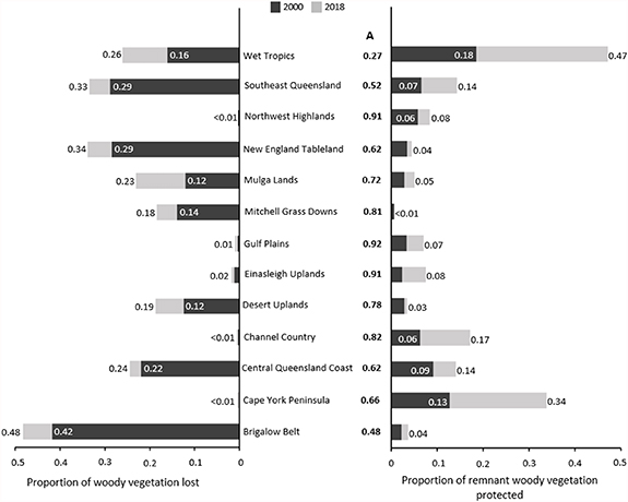

The coverage of remnant woody vegetation inside PAs has also been uneven across the state’s bioregions (figure 2). As of 2018, only the Cape York Peninsula and Wet Tropics had more than 30% of their remaining woody vegetation formally protected. These were also the two bioregions where most protection gains occurred between 2000 and 2018. In contrast, most other bioregions, including the Brigalow Belt, Mitchell Grass Downs, and Mulga Lands, remained with less than 10% of their woody vegetation falling within the protected area network.

3.3. Woody vegetation loss and protection across Queensland’s subregions

Historic patterns of woody vegetation loss across Queensland’s subregions varied widely (figure 3, table S2). Amongst the extremes, approximately 19% of the 116 assessed subregions record almost no vegetation loss, while 9% lost over 70% of their pre-1750 woody vegetation. More recently (between 2000 and 2018), 15 subregions lost more than 10% of their remnant woody vegetation, although 34 (29%) lost relatively little (<1%). Overall, subregions with high historical clearing tended to experience higher losses during the 2000–2018 period, with an average additional loss of 8% in those already heavily degraded. Subregions with the highest loss rates tended to be concentrated in a few bioregions, namely the Brigalow Belt, Mulga Lands, and Southeast Queensland. Considerable losses occured in the Wet Tropics, although over 90% of it attributed to natural disturbances.

Figure 3. Woody vegetation protection and losses in Queensland’s subregions. Change in clearing (predominantly by humans) and protection between 2000 and 2018 as a function of the percentage of remnant woody vegetation cleared (a) and protected (b) by 2000. (c) Map of the proportion of loss relative to gains in Queensland’s subregions between pre-clearing years and 2018, expressed as the metric F (F approaches 1 with increasing protection relative to loss and approaches −1 with decreasing protection relative to loss). (d) Map of the proportion of loss relative to gains in Queensland’s subregions between 2000 and 2018, expressed as the metric M (like F; M approaches 1 with increasing protection relative to loss and approaches −1 with decreasing protection relative to loss). Inset maps correspond to the Wet Tropics and the Central Queensland Coast. Bioregion boundaries are delineated in bold, and subregions not included in the analysis are grey.

Download figure:

Standard image High-resolution image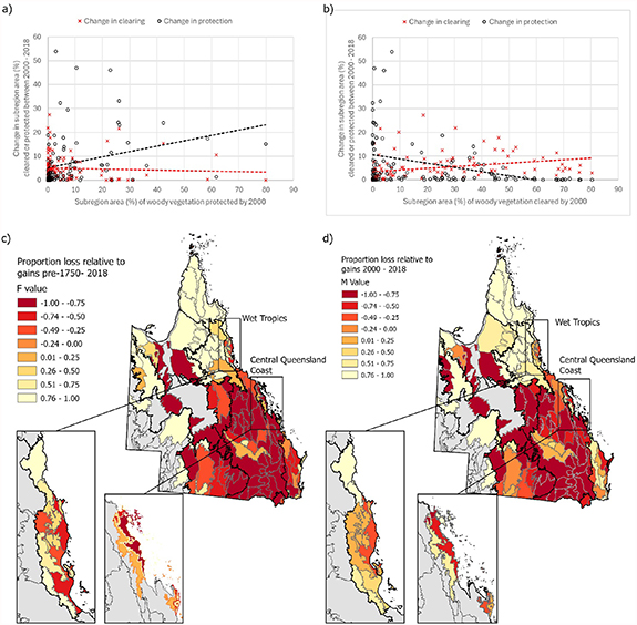

Protection efforts also varied substantially. The most significant gains occurred in subregions within Cape York Peninsula and the Wet Tropics, where more than half had over 30% of their woody vegetation under protection by 2018, increasing from very low protection levels in 2000 (figure 3, table S2). However, in much of the state, including the Brigalow Belt, Mitchell Grass Downs, Desert Uplands, and Mulga Lands, protected area coverage remained extremely low. By 2018, nearly two-thirds of subregions still had less than 10% of their woody vegetation protected, and only 15% had exceeded a 30% threshold.

3.4. Relationship between woody vegetation loss and protection

Most of Queensland’s subregions experienced high rates of loss alongside relatively low rates of protection as of 2018 (figures 3(a) and (b)), predominantly occurring within the Brigalow Belt, Southeast Queensland, and Mulga Lands bioregions (figures 3(c) and (d)). In contrast, subregions with high protection and low loss were concentrated almost entirely in the Cape York Peninsula. Some areas, like parts of the Wet Tropics, showed a mixed pattern of high loss (most from natural disasters) and high protection, underscoring the importance of considering both pressures simultaneously. Between 2000 and 2018, only 40% of the subregions gained more protection than they lost in vegetation, while 70 subregions (60%) saw greater losses than protection gains.

Subregions with major vegetation loss by 2000 tended to continue losing vegetation at higher rates after that year (figure 3(a), p < 0.05). Likewise, subregions with more protection in place in 2000 were also more likely to receive additional protection by 2018 (figure 3(b), p < 0.05), suggesting that conservation efforts have often reinforced existing spatial biases rather than counteracting risk.

3.5. Risk status of subregions

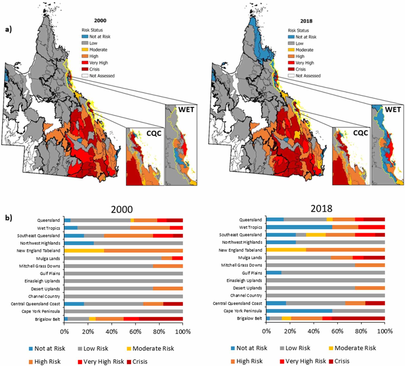
By 2018, only 14.7% of Queensland’s subregions were ‘Not at Risk,’ with a further 41.4% falling into low or moderate categories. The remaining 44% were classified as high or very high risk (table 2). Risk status remained unchanged in most subregions (n = 90) between 2000 and 2018. Improvements occurred primarily among subregions initially at low or moderate risk, with only two improving from high to moderate, both in Southeast Queensland (figure 4). In contrast, seven subregions already at high or very high risk in 2000 declined further, all in the Brigalow Belt and Mulga Lands, except Tully in the Wet Tropics. Six others shifted from low to higher risk, again concentrated in the Brigalow Belt and Mulga Lands, underscoring the continued spread of vegetation loss in areas with limited protection.

Figure 4. Subregion risk status as of 2000 and 2018 shown spatially (a) and proportionally within each bioregion (b). Risk status was defined in terms of the overall proportion of woody vegetation lost and the ratio of proportion lost to proportion protected ‘F’ [F = (%protected—%loss)/(%—%loss)] for each subregion. Bioregion boundaries are delineated in bold (a). Zoomed to Wet Tropics (WET) and Central Queensland Coast (CQC), highlighted by yellow boundaries (a). Subregions with <33.33% woody vegetation cover were not assessed (n = 16).

Download figure:

Standard image High-resolution image

Table 2. Changes in subregion risk status from 2000 to 2018. Risk status was defined in terms of the overall proportion of woody vegetation lost and the ratio of proportion lost to proportion protected for each subregion.

2018 Risk Status Not at riskLowModerateHighVery highCrisisTotal 2000 Risk StatusNot at risk6—————6 Low1142141—59 Moderate——3———3 High——2182123 Very High————549 Crisis—————1616 Total1742622821116

A positive trend was observed in Cape York Peninsula, where several low-risk subregions improved to ‘Not at Risk’ status by surpassing 30% protection (figure 4(b)). A similar pattern occurred in the Wet Tropics, though only among low-risk subregions; higher-risk areas showed no improvement. Tully, in fact, worsened to very high risk by 2018.

Only a few subregions were classified as moderate risk in both 2000 and 2018 (table 2), highlighting a regional polarisation; most subregions experienced either extensive clearing with little protection or relatively little clearing overall. Subregions that were high risk in 2000 generally saw lower protection gains and higher continued loss than those at lower initial risk. These patterns were especially evident in the Brigalow Belt and Mulga Lands (figure 3(d)).

Summary statistics for rates of loss and protection, woody vegetation extent, and risk status for bioregions and subregions are provided in tables S1 and S2, respectively.

Our analysis shows that Queensland has lost 21.4% of its original woody vegetation since European colonisation, with only 9.6% currently protected. Although the area under formal protection more than doubled between 2000 and 2018, one-fifth of all historical loss also occurred during this period. Importantly, a clear spatial mismatch emerged: regions with historically high clearing continued to lose vegetation with little or no protection gains, while gains were concentrated in already well-protected, low-loss regions, a pattern reported globally (Joppa and Pfaff 2009, Watson et al 2016). Consequently, risk status remained unchanged for nearly 80% of subregions between 2000 and 2018. Only a small share of subregions improved (9% in terms of overall risk and 11% in protection gains), highlighting limited conservation progress in Queensland when considering rates of loss versus protection. These findings align with evidence that Queensland has the nation’s highest rate of threatened species habitat loss (Ward et al 2019) and has recovered only four federally listed species in the past 20 years, all from far north Queensland (Ward et al 2024).

Our study illustrates that evaluating gains versus losses is important for assessing conservation outcomes. For example, the Wet Tropics had the highest proportion of protected woody vegetation but also experienced substantial vegetation loss (albeit from natural disturbance), showing that high protection does not equate to no losses. Southeast Queensland and the Central Queensland Coast showed similar mismatches. Furthermore, our subregional analysis reveals that within these bioregions, protection and loss are unevenly distributed. In many cases, protection gains occurred in only a few subregions, while others remained largely unprotected. These cases highlight the importance of evaluating conservation outcomes at finer spatial scales to avoid misleading conclusions about regional progress.

Regional disparities were especially pronounced in the Brigalow Belt, which emerged as a ‘Crisis’ bioregion. As one of Australia’s most heavily cleared and fragmented landscapes (Accad et al 2024, Queensland Government 2018), it continued to undergo some of the highest rates of woody vegetation loss after 2000, with several subregions exceeding 70% loss. Yet less than 4% of the bioregion’s woody vegetation was formally protected, leaving many subregions in the highest risk categories. This is concerning given that up to 92% of the Brigalow Belt’s remnant vegetation is of state or regional significance (Queensland Government 2018). Similar dynamics were observed in the Mulga Lands and Southeast Queensland, where subregions with extensive historical loss continued to experience clearing with minimal protection gains. These landscapes support threatened and endemic species, threatened ecological communities, and species’ irreplaceable habitats (Neldner et al 2017, Hernandez et al 2024, Ward et al 2025). In contrast, some Wet Tropics subregions and much of Cape York Peninsula had higher initial protection and received the most gains between 2000 and 2018. This pattern is consistent with evidence that conservation investments often favour regions with lower opportunity costs or political resistance rather than those with the most urgent ecological need (Venter et al 2018, Visconti et al 2019).

While some subregions showed improved risk status, most (particularly those already at high risk) remained static or worsened between 2000 and 2018. These findings align with the ‘residual protection’ concept, where PAs are established on less threatened or lower-value lands (Pressey and Tully 1994, Joppa and Pfaff 2009, Venter et al 2018). This pattern reflects underlying drivers, including spatial biases in PA placement, high agricultural opportunity costs, and ongoing pressures from grazing, cropping, and mining. These threats are compounded by inconsistent amendments, weak enforcement, and non-compliance under policies regulating clearing (Evans 2016, State of Queensland 2023, Thomas et al 2025). PAs provide benefits beyond preventing habitat loss (Stolton et al 2015, Watson et al 2023) but their limited expansion in heavily cleared regions has constrained their effectiveness (Hernandez et al 2021). Conservation success in Queensland requires stronger integration of PA expansion, clearing controls, and restoration. This is especially relevant if a truly representative, adequate, and comprehensive National Reserve System, the goal of the Commonwealth Government (National Resource Management Ministerial Council 2009), is to be established.

The risk classification framework used here provides a valuable tool for evaluating conservation needs. For example, subregions in ‘crisis’ or at ‘very high risk’ should be prioritised for policy interventions, such as land clearing moratoriums, habitat restoration, and targeted protected area expansion. Subregions such as Callide Creek Downs and Dawson River Downs, with >70% vegetation loss and minor protection, represent urgent cases. Conversely, subregions currently at low or no risk should only be prioritised if they contribute to broader goals, such as those quality components from the Global Biodiversity Framework’s target 3, including connectivity, ecosystem function and services, or areas of particular importance for biodiversity (Watson et al 2023). While our study focuses on Queensland, the approach and findings have broader implications for global conservation policy, as many countries report progress toward biodiversity targets using protected area expansion alone, often without accounting for concurrent habitat loss.

We acknowledge our analysis excluded vegetation regrowth, which can aid ecosystem recovery over time (Bowen et al 2007, Crouzeilles et al 2016, 2017). However, regrowth is rarely equivalent to intact remnant habitat when considering its biodiversity and ecosystem service values (Lindenmayer et al 2011). In Queensland, this could take several decades (Thomas et al 2025). However, future studies could incorporate regrowth dynamics more explicitly, particularly given the GBF’s emphasis on restoring degraded ecosystems and ecological integrity. Furthermore, although our biennial PA data inherently capture net changes in extent, including downsizing and degazettement events, we did not explicitly differentiate these (or for downgrades) as reported in other datasets (Cook et al 2017). Available evidence suggests such events comprise only a small fraction of Queensland’s PA estate, but future research should examine them more directly, especially at finer temporal scales where localised losses may be more consequential (Cook et al 2017).

Finally, our analysis ends in 2018 due to changes in SLATS methodology that limit comparability with more recent data. We note that recent SLATS reports indicate that clearing has continued in high-risk bioregions such as the Brigalow Belt and Mulga Lands since 2018 (Queensland Department of Environment and Science 2024). Moreover, there have been limited gains in protection across the state since 2018, suggesting that the issues highlighted in this study are ongoing. If national targets under the Global Biodiversity Framework (CBD 2022) are to be met, a shift in conservation strategy is required. This includes rebalancing protection efforts toward high-risk regions, implementing stricter controls on land clearing, and investing in restoration where remnant habitat has already been heavily depleted.

Our analysis reveals an imbalance between habitat loss and protection across Queensland, highlighting significant deficiencies in biodiversity conservation strategies. A more nuanced and spatially explicit approach is needed to actively prioritise regions most under threat for protection, enforcement, and restoration. Without these decisive actions, Queensland risks continued biodiversity loss, compromising ecosystem resilience and international conservation obligations. Global indicators such as the Species Habitat Index (GEO BON 2021) provide complementary perspectives at the species level, but our focus here has been on land-cover balance sheets that directly track protection and loss across space and time.

We thank two anonymous reviewers for their helpful comments.

All data that support these findings are available to download through repositories from the Queensland Government, including https://qldspatial.information.qld and www.data.qld.gov.au/. Used datasets are listed in the supplementary materials.

The data that support the findings of this study are openly available at the following URL/DOI: https://qldspatial.information.qld.gov.au/catalogue/.

Vegetation Change Queensland available at https://doi.org/10.1088/1748-9326/ae1623/data1.

The authors declare that they have no competing interests.