1748-9326/20/11/114085

Abstract

Although precipitation increases have been observed in different areas of the globe and at various temporal resolutions, changes in precipitation can be difficult to detect and attribute to anthropogenic forcing in observational records due to the significant influence of natural variability. Here, we quantify the influence of large-scale atmospheric circulation variability on total winter precipitation for Europe using dynamical adjustment with synoptic-scale weather patterns (WPs). Variability in atmospheric dynamics, through frequency changes in WPs, is shown to be a significant driver of observed wetting and drying trends, linked to observed trends in the North Atlantic jet stream. After removing dynamical variability, trends emerge in non-dynamical winter precipitation which are attributable to anthropogenic forcing: a north-south signal of a drying Mediterranean and increasingly wetter mid-to-high latitudes. Although this spatial pattern is well-represented by CMIP6 models, the magnitude of observed changes is approximately 23 years ahead of the CMIP6 multi-model mean predictions. Our results suggest that current adaptation strategies, based on multi-model means, may underestimate the near-term risk of climate-related hazards, and therefore require critical re-evaluation.

Export citation and abstractBibTeXRIS

Understanding changes to seasonal precipitation variability is critical for climate change adaptation and mitigation. Precipitation extremes cause floods and landslides, while longer-term changes affect water resources, agriculture and carbon sequestration (Lloyd et al 2024). Detecting and attributing these changes is challenging due to the substantial influence of natural variability on precipitation (Deser et al 2017, Ballinger et al 2023).

Natural variability can mask externally-forced signals, complicating efforts to identify emerging trends (Deser et al 2012, Fereday et al 2018). Despite this, there is growing observational evidence of a north-south pattern in European winter precipitation changes: intensifying rainfall in the mid-to-high latitudes and drying in the Mediterranean (Knutson and Zeng 2018, Guo et al 2019, Ossó et al 2022, de Vries et al 2023). Some of these trends have been attributed to anthropogenic warming (Christidis and Stott 2022, Ballinger et al 2023). Model projections suggest that robust climate signals in European mean precipitation should not emerge until around the middle of the 21st Century (Zappa et al 2015, Deser et al 2017, Wood and Ludwig 2020, Christidis and Stott 2022, Ballinger et al 2023). Yet, the magnitude of observed trends in precipitation often exceed those simulated by climate models (Knutson and Zeng 2018, Wehrli et al 2018, Baker et al 2019, Moreno-Chamarro et al 2021).

Whether this disparity is due to incorrect modelled responses to external forcing or due to natural variability is not clear, particularly since observed changes in large-scale atmospheric circulation are poorly understood. The recent strengthening of the winter North Atlantic Oscillation (NAO) is not captured by CMIP6 models (Blackport and Fyfe 2022 and the disparity between historical observed and modelled trends of Northern European winter precipitation can be reduced by accounting for the influence of the NAO (Ballinger et al 2023). Yet, the fact that biases remain after accounting for large-scale dynamics indicates that the thermodynamical response of precipitation in climate models is likely too weak. To understand model biases in their responses to external forcing, disentangling dynamic and thermodynamic processes in both observations and models is crucial (Wehrli et al 2018).

In this study, we use a dynamical adjustment methodology to disentangle dynamical and non-dynamical contributions to observed precipitation trends in Europe over 1950–2024. Dynamical adjustment methodologies leverage the statistical relationships between atmospheric circulation patterns and surface weather phenomena derived from long observational records (Deser et al 2016, Guo et al 2019). We compare trends obtained from observational datasets with those from an ensemble of CMIP6 climate models, focussing on the representation of the non-dynamical component.

We address three key questions:

1.

How has winter precipitation changed since 1950 in Europe?

2.

To what extent can changes in winter precipitation be attributed to dynamical variability and anthropogenic forcing?

3.

What are the physical explanations for the observed changes in winter precipitation?

2.1. Observed and modelled precipitation data

Observed daily precipitation data comes from ERA5 and EOBs for 1950–2024 and from four national datasets (UK: HadUK-Grid, Ireland: Met Éireann, Germany: HYRAS and Netherlands: KNMI) for the period 1950–2014.

Attribution is conducted using a suite of CMIP6 experiments. Historical all forcing simulations (1950–2015) were extended with SSP2-4.5 simulations (2015–2020) (CMIP6-historical) and historical natural forcing only models (CMIP6-natural) for 1950–2020 were accessed. To establish a baseline for pre-industrial internal variability, we also used the ensemble of pre-industrial control experiments (CMIP6-control). From these control experiments, a distribution of plausible 70 year trends is generated by taking 1000 random, continuous 70 year segments sampled from their time series. Trends are then calculated for each of these 1000 segments, forming the control/pre-industrial trend distribution. Models used are listed in the Supplementary Information.

2.2. Dynamical adjustment

The methodology is based upon that of Fereday et al (2018) and utilises a daily timeseries of 30 synoptic-scale weather patterns (WPs) covering a North Atlantic and European domain (30 W, 30E, 35 S and 70 N). The WPs were developed by the UK Met Office and classified by K-means clustering of daily mean sea level pressure anomaly fields in the EMULATE dataset for 1850–2010 (Neal et al 2016). These WPs have been designed with expert elicitation to capture the dominant modes of variability over Western Europe and as such are appropriate for this work. It should be noted that other clustering methodologies are available for defining WPs (i.e. self-organising maps (Lennard and Hegerl 2015) or weather-type optimisation (Serras et al 2024)).

The dataset has been extended to 2024 using a combination of ERA-Interim and ERA5 reanalysis. It should be noted that in other seasons and at shorter timescales, the suitability of this dynamical adjustment methodology is diminished due to the weaker influence of synoptic-scale systems on European precipitation (Fereday et al 2018).

To assess changes to accumulated seasonal precipitation, we first remove the dynamic contribution to precipitation from each precipitation dataset by applying the same method over the given domain and available time period:

1.

Bin 1950–1980 daily precipitation by WP and month. (Other sampling periods are tested and show limited effect on results, see supplementary information).

2.

Create 1000 synthetic rainfall timeseries based on the observed 1950–2024 WP time-series using a bootstrap approach, resampling different daily rainfall amounts from the pool of appropriate WP and month.

3.

Aggregate the 1000 daily time-series into seasonal time-series.

4.

Calculate the average of the 1000 seasonal timeseries, providing the best estimate of the expected seasonal precipitation for 1950–2024 based on dynamical variability characterised from WPs—‘dynamical precipitation’.

5.

Calculate the difference between the seasonal observed and dynamical precipitation—this represents the amount of observed precipitation above or below what was expected from WP dynamics that season—‘non-dynamical precipitation’.

This dynamical adjustment methodology above is applied to ERA5 and EOBs, as well as the national datasets (1950–2014) and CMIP6-natural and CMIP6-historical (1950–2020). For all these datasets, the period for step one (1950–1980) is the same. For CMIP6-control, the same methodology is performed but without setting a cutoff date of 1980.

The number of WPs and variability of synoptic conditions represented gives us confidence this dynamical adjustment methodology captures the internal variability and any externally forced signal in dynamical precipitation. The non-dynamical precipitation component is therefore assumed to primarily represent thermodynamically-induced changes. However as Sexton et al (2024) also raise, there is the possibility that some dynamical processes at the sub-domain scale may be conflated with thermodynamical processes in the non-dynamical component. This will be discussed further in the results.

2.3. Attribution methodology

For the spatial pattern attribution, we calculate the ensemble mean trend from the CMIP6-historical and CMIP6-natural simulations for the 1950–2020 period. Attribution to anthropogenic forcing is inferred if two conditions are met:

1)

The spatial correlation between the observed non-dynamical precipitation trends and the CMIP6-historical ensemble mean falls outside the 5–95th percentile range of the spatial correlations found within the internal variability distribution derived CMIP6-control

2)

The spatial correlation between the observed non-dynamical precipitation trends and the CMIP6-natural ensemble mean falls within the 5–95th percentile range of the spatial correlations found within the internal variability distribution derived CMIP6-control.

This would indicate that the observed spatial pattern of trends is statistically unlikely to have occurred without the influence of external (anthropogenic) forcing.

Grid cell attribution is conducted based on the methodology of Knutson and Zeng (2018). At each grid cell, we calculate the distribution of trends from individual members of the CMIP6-historical and CMIP6-natural ensembles for the 1950–2020 period. Observed trends are then assessed against two criteria:

1)

An observed trend is deemed attributable to anthropogenic forcing if it falls outside the 5–95th percentile range of the CMIP6-natural trend distribution but remains within the 90th percentile of the CMIP6-historical trends.

2)

Additionally, trends which are higher (or lower) than both the 5–95th percentile range of natural and historical simulations but are of the same sign as the historical mean trend are deemed attributable to anthropogenic forcing, with the model simulations showing a bias towards weaker trends.

2.4. Time of emergence methodology

The gridcell signal to noise ratio (S/N) in observations and CMIP6-historical is estimated using the methodology from Hawkins et al (2020). Non-dynamical precipitation is regressed onto annual mean global mean surface temperature (GMST) smoothed with a 41 year loess filter to isolate the long-term changes in temperature:

where P(t) is the regression model predicted precipitation at time t, GMST(t) is the smoothed GMST at time t, β is the linear scaling coefficient between P and GMST, and α is a constant. At any given year t, the signal which has emerged at that year is P(t)-P(1950), where P(1950) is the first timestep in the series. The noise is calculated as the standard deviation of the residuals of the regression model. 90th confidence intervals for β are also calculated via bootstrap resampling with replacement. Time emergence is calculated as the first year where the S/N ratio increases above one standard deviation.

3.1. Comparison of data sources

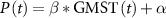
We first examine the trend in total winter precipitation over Europe from 1950 to 2024 (top row, figure 1). It should be noted that E-OBS has limited station coverage in some areas such as Portugal, Spain, Italy and Iceland, which can lead to interpolation errors and biases. On the other hand, ERA5 is a model-derived reanalysis product that is known to underestimate intense rainfall (Courty et al 2019, Guerreiro et al 2024), particularly in mountainous regions (Lavers et al 2022).

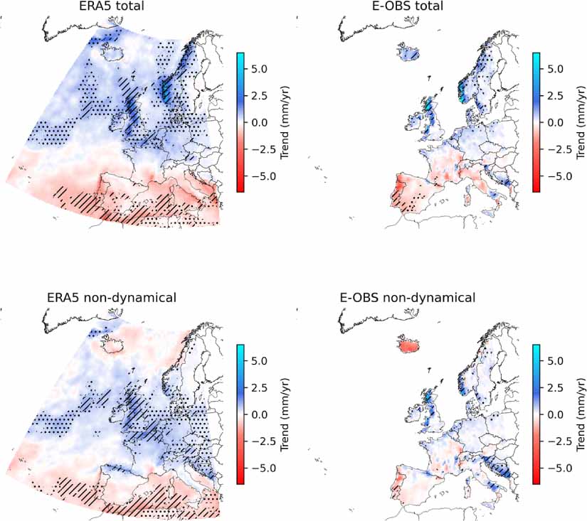
Figure 1. Observed trends from 1950 to 2024 in total observed, dynamical and non-dynamical winter precipitation for the European domain for ERA5 and E-OBS. Stippling indicates significance at the 90th confidence interval calculated via bootstrap resampling.

Download figure:

Standard image High-resolution image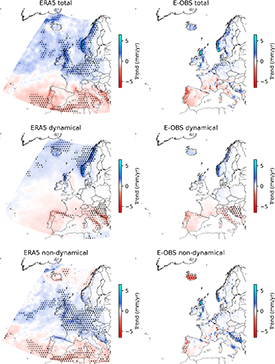

We find distinct spatial patterns of change, with increases in the mid-to-north latitudes and reductions in southern Europe, consistent with previous studies (Guo et al 2019, Christidis and Stott 2022, Ossó et al 2022). We find significant increases on the west coast of the British Isles, Norway and around Benelux. Statistically significant decreases in winter precipitation over land are not found in ERA5, and in E-OBS are mainly in Portugal. Overall, ERA5 exhibits lower trend magnitudes than E-OBS. In areas with the largest positive trends, such as in northwest Scotland, the increase in winter precipitation in ERA5 is approximately half that of E-OBS.

We also investigate trends using national-scale observational datasets for the UK, Ireland, the Netherlands and Germany. Figure S2 shows that there is closer agreement between the national datasets and E-OBS than with ERA5. In particular, the national datasets show significant non-dynamical trends over topography in the UK and a lack of significant trend over most of Germany, which are only present in ERA5. However, the spatial pattern of significant trends in the south-east of England and across the Island of Ireland are better captured by ERA5. Additionally, the magnitude of trends in E-OBS may be too high in places over topography in the UK. Another consideration is that the national-scale in-situ datasets also suffer from uncertainties. These results indicate that both ERA5 and E-OBS should be examined over the full timeseries.

3.2. Dynamical trends

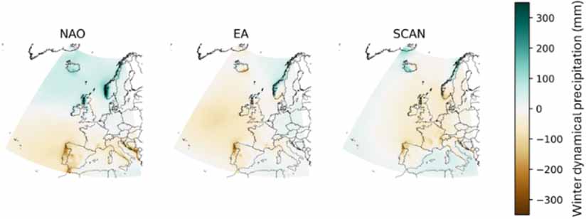
The spatial pattern of dynamical precipitation trends (figure 1, middle row) indicates increasing frequency of WPs associated with higher precipitation in the north of the domain, and particularly over the west coasts of the British Isles and Norway, and lower precipitation in the South of Europe. Figure 2 presents spatial maps of the regression coefficients from a multiple linear regression analysis relating winter dynamical precipitation, as the dependent variable, to three atmospheric indices: the North Atlantic Oscillation (NAO), East Atlantic pattern (EA) and Scandinavian pattern (SCAND). The observed increase in dynamical precipitation at high latitudes closely follows the pattern of positive NAO-induced dynamical precipitation, related to more frequent NAO-positive conditions since the 1950s (Ummenhofer et al 2017, Blackport and Fyfe 2022, Eade et al 2022). This may be caused by the observed poleward movement of the North Atlantic jet stream in winter (Woollings et al 2023), which is also projected in climate models (Rousi et al 2021), but the degree to which this is natural variability or externally-forced is unclear.

Figure 2. The effect of a one unit increase in North Atlantic Oscillation (NAO), East Atlantic pattern (EA) and Scandinavian pattern (SCAND) indices on winter dynamical precipitation in ERA5, as calculated with multiple linear regression.

Download figure:

Standard image High-resolution image

Reduced winter precipitation in southern Europe is a robust signal in climate models, predominantly driven by dynamical changes (Barcikowska et al 2018, Brogli et al 2019, Tuel and Eltahir 2020) causing increased anticylonic conditions over the eastern Mediterranean in future winters. In the west, regions such as the Iberian Peninsula are less directly affected by the emerging anticylonic conditions and precipitation declines are primarily driven by reduced moisture transport related to the poleward movement of the jet stream.

3.3. Non-dynamical trends

The spatial pattern of non-dynamical precipitation trends (bottom row of figure 1) aligns with the projected response of winter precipitation in Europe to anthropogenic forcing (Deser et al 2017, Christidis and Stott 2022).

The most significant upward trends are in northwest Europe at the exit of the North Atlantic storm track. The winter climatology of precipitation from atmospheric rivers (ARs) and extra-tropical cyclones (ETCs) in Europe (Hawcroft et al 2012, Lavers and Villarini 2015) closely matches the observed wetting pattern, thus it is likely due to additional moisture and precipitation from transiting ETCs. A secondary area of non-dynamical wetting along the Balkan coastline also receives over 75% of its winter precipitation from ETCs (Hawcroft et al 2012). Precipitation in ETCs and ARs is robustly linked to temperature increases due to high moisture availability, saturated water vapour pressure and dynamical feedbacks within these systems (Catto et al 2019, Berthou et al 2022). Climate models project precipitation intensity from ETCs and ARs will increase in NW Europe, in the same region as the observed non-dynamical intensification (Lavers et al 2013, Gao et al 2016, Hawcroft et al 2018).

We find a significant negative trend in non-dynamical precipitation in both ERA5 and E-OBS over Portugal. The primary reason for this appears to be the poleward shift of storm tracks and ETCs, but this drying is further enhanced by increased atmospheric stability, which impedes the conversion of available moisture into rainfall (Fernández-Alvarez et al 2023).

Precipitation trends in ERA5 over the oceans should be interpreted with caution due to the lack of observational data for validation; however, increases in non-dynamical precipitation in the mid-latitudes and decreases in the sub-tropics align with the ‘wet gets wetter, dry gets drier’ theory. The reduction of precipitation in the high latitudes, from the Greenland Sea to the coast of Norway, may be explained by the North Atlantic Warming Hole, which has been shown in climate models to produce a reduction in mean winter precipitation in a similar area, partially due to limited moisture transfer to the atmosphere and increases in static stability (Hand et al 2019, Iversen et al 2023).

Figure 3 illustrates the CMIP6 ensemble mean trends in total, dynamical, and non-dynamical winter precipitation for the period 1950–2024, with individual CMIP6 model trends presented in figures S4–S6. Most models project increasing precipitation in northern Europe and decreasing precipitation in the south. The precise geographical areas experiencing these trends, along with their magnitudes, vary considerably amongst models.

Figure 3. 1950–2024 CMIP6 ensemble multimodel mean trends (mm yr−1) for total, dynamical and non-dynamical winter precipitation over Europe. Stippling indicates where trends are outside the 90th confidence interval of ensemble mean control run trends. The stippling for total and non-dynamical trends indicate the presence of externally forced trends in these components.

Download figure:

Standard image High-resolution image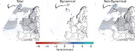

In observations, a substantial component of the spatial pattern is driven by dynamical changes, reflecting the observed strengthening of the jet stream and a trend towards NAO-positive conditions. This is also largely true for most models, where the magnitudes of non-dynamical precipitation changes are considerably smaller.

Figure 3 reveals that when these spatially heterogeneous model trends are averaged into a multi-model mean, their differing signals largely cancel each other out. Consequently, the resulting changes are an order of magnitude smaller than those found in observations or within individual models. In this multi-model mean, changes in total precipitation primarily stem from the non-dynamical component. This result confirms that multimodel means are not suitable for assessing changes to either total or dynamical precipitation, and their use will mask the physical drivers of the individual model changes.

The non-dynamical component of precipitation, which largely represents the thermodynamic response, should theoretically be comparable across models, as the main drivers of natural variability are predominantly captured by the dynamical portion. However, figure S6 shows that non-dynamical trends across different models still vary in magnitude and spatial pattern. Some models exhibit magnitudes and patterns of trends broadly similar to observations, while others show very different spatial patterns of trends or exhibit a complete lack of significant trends.

We note that aggregating the varied spatial pattern in different models cancels out some trends in the multimodel mean. As a result, multimodel mean trends in non-dynamical winter precipitation are an order of magnitude lower than the trends in observations and some individual climate models.

Nevertheless, the 1950–2024 multimodel mean non-dynamical trend exhibits a distinct spatial pattern that cannot be attributed solely to internal variability (figure 3), and captures the expected spatial response to anthropogenic forcing. Extending the analysis period forwards to 1950–2099 enhances the influence of anthropogenic forcing and reveals far greater consistency among models (figure S7). These show broad agreement with the spatial pattern of the 1950–2024 multimodel mean trend.

4.1. Attribution of spatial patterns of non-dynamical trends

We conduct attribution of non-dynamical winter precipitation trends, both for spatial patterns and grid-cell changes, by comparing observed trends against the anthropogenic signal from CMIP6 historical/SSP2-4.5 simulations. The significance of this comparison, relative to natural forcing only and internal variability, was assessed using CMIP6 natural forcing only simulations and pre-industrial control runs respectively. The following analysis assesses the spatial pattern of 1950–2020 trends in the non-dynamical component.

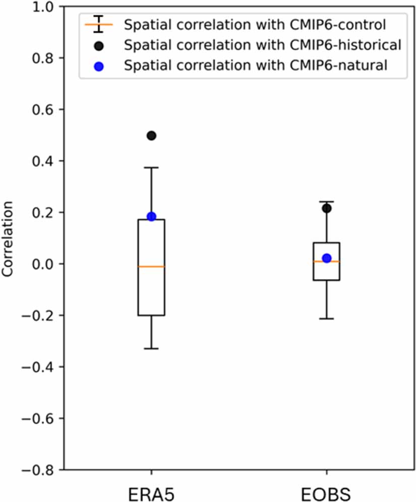
The spatial correlation of trends between ERA5 and the CMIP6-historical multimodel mean exceeds the 95th percentile of correlations between ERA5 and the CMIP6-control multimodel mean distribution (figure 4). This indicates that the spatial pattern of non-dynamical winter precipitation trends in ERA5 is extremely unlikely to have arisen from internal variability alone. For E-OBS, the non-dynamical trend pattern is very unlikely to have occurred due to internal variability alone, with the CMIP6-historical correlation being at the 93rd percentile of CMIP6-control correlations. Correlations with the CMIP6-natural multimodel mean are lower for both ERA5 and E-OBS than correlations with CMIP6-historical, indicating that the spatial pattern of observed trends more closely resemble the modelled response to anthropogenic warming than natural forcings alone. These results mean that the spatial pattern of European winter non-dynamical precipitation trends is attributable to anthropogenic climate change.

Figure 4. Spatial correlation between the observed 1950–2020 trends with modelled trends with historical forcing, natural forcing only and pre-industrial control simulations. Points indicate the spatial correlation coefficient for non-dynamical winter precipitation trend pattern in ERA5 and E-OBS with CMIP6-historical (black) and CMIP6-natural (blue) non-dynamical precipitation ensemble mean trend pattern (both 1950–2020). Boxplots indicate the 5–95th percentile range of correlations with CMIP6-control non-dynamical precipitation ensemble mean trend patterns.

Download figure:

Standard image High-resolution image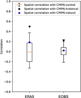

When the attribution is repeated for total winter precipitation, spatial correlations of ERA5 and EOBS trends with CMIP6-historical trends both fall within the 5–95th percentile range of correlations with control trends (figure S8). The spatial pattern of total precipitation trends is therefore not attributable to anthropogenic warming. Relying on analysis of total precipitation trends would lead to the incorrect conclusion that the spatial pattern of observed changes to winter European precipitation is not attributable.

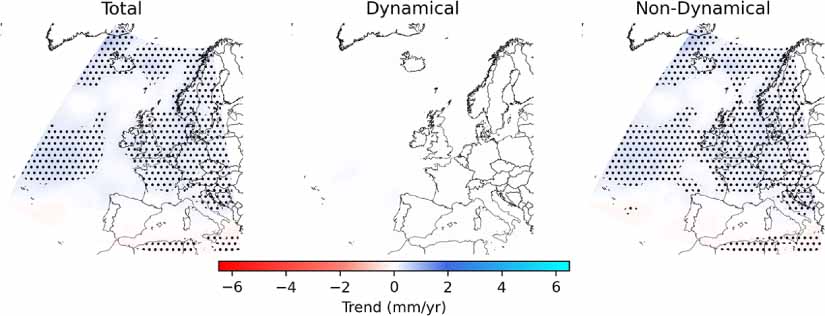
4.2. Grid cell attribution

We can also show how accounting for dynamical variability improves attribution in non-dynamical precipitation compared to total precipitation at the grid-cell level (figure 5). We attribute grid-cell level trends in total and non-dynamical winter precipitation based on the methodology of Knutson and Zeng (2018). For non-dynamical winter precipitation, the main area of attributable wetting trends in ERA5 is shifted equatorwards compared to the wetting trend in total winter precipitation. We do not find widespread attributable wetting trends in E-OBS winter precipitation across Western and Central Europe. Both ERA5 and E-OBS indicate attributable non-dynamical winter precipitation drying trends in Portugal.

Figure 5. Grid-cell level attribution of observed trends in total and non-dynamical winter precipitation. Dotted hatching indicates where observed trends are outside the 90th confidence intervals of CMIP6 natural forcing runs but inside the 5–95th percentile range of CMIP6 historical experiments. Diagonal hatching indicates where trends are outside the 5–95th percentile range of both CMIP6 natural forcing and historical experiments.

Download figure:

Standard image High-resolution image

The comparison between non-dynamical winter precipitation trends in both observations and CMIP6-historical is essentially a like-for-like comparison. For both ERA5 and E-OBS, the trends in non-dynamical winter precipitation for much of the UK, northern France and Belgium are greater than the 95th percentile of CMIP6 historical trends. This is also the case for the Balkans in E-OBS and, with a smaller spatial extent, in ERA5. As discussed earlier, most winter precipitation in both these regions originates from ETCs and ARs. Discrepancies between observed and modelled trends may be due to the representation of precipitation processes within these systems.

We find non-dynamical drying trends in winter precipitation for Portugal in E-OBS below the 5th percentile of non-dynamical drying trends in CMIP6-historical. Finally, ERA5 indicates winter drying across the Mediterranean Sea which is of significantly greater magnitude than the climate model simulations.

Our results indicate that while the CMIP6 models represent a spatial pattern of response in external forcing consistent with observed trends, they significantly underestimate the magnitude of these trends locally. Of grid cells with non-dynamical trends attributable to climate change in ERA5 and EOBS, 40% and 49% respectively have trend magnitudes outside the 5–95th percentile range of the CMIP6 models.

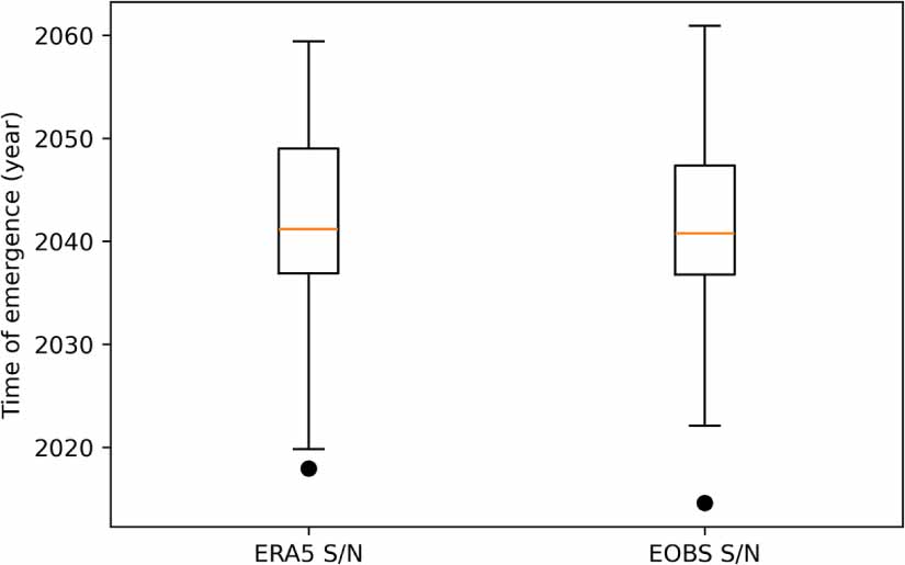
4.3. Time of emergence of non-dynamical precipitation signal

Figure S9 shows the S/N in 2024 of ERA5 and EOBS non-dynamical winter precipitation, highlighting grid cells with a S/N > 1. These grid cells can be said to show a robust S/N by 2024. On average, the time of emergence of a S/N > 1 in these grid cells is 2017 and 2014 for ERA5 and EOBS respectively.

We then calculate the same grid-cell S/N per ensemble member for the CMIP6 historical + SSP245 and extract the time of emergence of a S/N > 1 in the models at gridpoints with an observed emerged signal (i.e. gridcells with stippling in figure S9). The mean time of emergence across the ensemble is 2041 and 2040 for grid cells in ERA5 and E-OBS respectively. Figure S10 shows the spatial distribution of the CMIP6 ensemble mean S/N > 1 time of emergence, with a generally uniform emergence between 2030 and 2050.

There is a wide spread in the mean time of emergence across the CMIP6 ensemble, ranging from the 2010s to the 2060s (figure 6). The signal appears in observations 23 years earlier than the multi-model mean and most CMIP6 models (defined here by their interquartile range) suggest these signals should not have emerged until between 2035 and 2045.

Figure 6. CMIP6 average time of emergence of S/N > 1 for non-dynamical winter precipitation in gridcells with observed S/N > 1 in ERA5 and EOBS. The observed average time of emergence is plotted as a solid black circle. The box plots show the 5–95th percentile range.

Download figure:

Standard image High-resolution image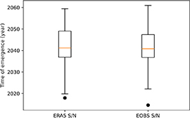

Our results emphasise the importance of accounting for large-scale dynamics when assessing changes in seasonal precipitation. We show that attributing total winter precipitation changes with a multi-model ensemble mean can produce a misleading attribution statement as differing dynamical trends across individual models may effectively cancel each other out within the multimodel mean. We also show that the non-dynamical winter precipitation component more closely aligns with the modelled response and attributing this component produces more reliable attribution statements.

In this sense, we are attributing changes in the component of winter European precipitation that we expect to observe, given the modelled response to external forcing. Since CMIP6 models do not simulate the observed intensification of the North Atlantic jet stream without an emergent constraint (Smith et al 2025), the dynamical component of winter European precipitation should be discarded when making attribution statements. Ballinger et al (2023) also show for European precipitation trends how accounting for variability in the NAO affects the calculation of biases in modelled precipitation trends. Our attribution results from dynamical adjustment are coherent with those found by Guo et al (2019) for precipitation and Lehner et al (2017) for temperature.

The attribution of trend patterns is dependent on the observational dataset used. However, while the E-OBS spatial pattern of trends is not formally attributable, it is still unlikely to have occurred without anthropogenic forcing and this gives confidence that the strong attribution statement for ERA5 is not due to spurious trends in the reanalysis model. The difference is possibly due to the limited station density in E-OBS.

While the spatial pattern of non-dynamical trends in winter precipitation in the CMIP6 multimodel mean does reproduce the observed pattern of trends, we show that the multimodel mean severely underestimates the magnitude of observed trends compared to ERA5 and E-OBS. The results here add to the evidence that coarse-resolution global models tend to underestimate the observed intensification of precipitation adequately, even at seasonal timescales (Knutson and Zeng 2018). GCM-class climate models do not physically simulate many processes which are important for precipitation (i.e. convection and orographic enhancement) and precipitation–temperature–humidity coupling has been shown to be better represented in high resolution convection permitting models (Lenderink et al 2025).

Using the ensemble mean, which is typically used to derive the influence of external forcing, CMIP6 models show a n intensification of winter precipitation which is approximately 23 years behind the observed trend. These findings have important implications for the urgency and scale of adaptation decisions, since the attributable climate signal in winter precipitation in Europe appears to be emerging much faster than GCMs have projected so far. In particular, this will mean that future winter flood risk, particularly in northern Europe, is substantially underestimated by GCMs and that risk is already higher than these models suggest. Further work is required to better understand changes in other seasons.

JGC wais funded by the OnePlanet NERC DTP (NE/S007512/1) and the Willis Research Network. HJF was supported by the Co-Centre for Climate + Biodiversity + Water funded by UKRI (NE/Y006496/1). SBG is NUAcT Fellow. We thank the anonymous reviewers as well as Professor Peter Stott, Dr Stephen Blenkinsop and Dr Leanne Wake for their useful comments on this work.