The year is 2025, and the data engineering landscape has never been more exciting—or more confusing. Walk into any tech conference, and you’ll hear buzzwords flying around like “lakehouse,” “Delta Lake,” “Iceberg,” and “unified analytics.” But beneath all the marketing noise lies a fundamental question that keeps data architects awake at night: Which platform can actually deliver on the promise of fast, reliable, cost-effective analytics at scale?

To answer this question, we embarked on the most comprehensive benchmark we could design: 1TB of industry-standard TPC-H data, 8.6 billion rows, and two of the most talked-about platforms in modern data engineering going head-to-head in an epic performance showdown.

This isn’t another vendor shootout. We’re comparing two different takes on data architecture—one with UC Berkeley roots, one from Netflix’s open‑source world—to see how they perform in practice.

Buckle up. We’re about to dive deep into the technologies that are reshaping how the world thinks about data.

Chapter 1: The Genesis Stories - How Giants Are Born​

Databricks: From Academic Research to Enterprise Dominance​

Born out of UC Berkeley’s AMPLab, Spark set out to make distributed computing actually usable. In 2013, its creators launched Databricks to turn that power into something teams could run day to day—first as managed Spark, then as a full platform.

Highlights, at a glance:

• 2013–2015: Managed Spark + notebooks.
• 2016–2018: Cluster automation, collab notebooks, early MLflow.
• 2019–2021: Delta Lake brings ACID, schema enforcement, time travel.
• 2022–2025: Unity Catalog, Photon, tighter AI/LLM workflows.

Net-net: Databricks evolved from “Spark‑as‑a‑service” into a unified analytics platform focused on speed, reliability, and usability.

Apache Iceberg: The Open Source Rebellion​

While Databricks doubled down on an integrated platform, Netflix, Apple, and LinkedIn hit classic data‑lake pain: tiny files, slow planning, brittle schema changes—and growing discomfort with vendor lock‑in.

How Iceberg showed up:

• 2017: Netflix kicked off Iceberg to fix those fundamentals.
• 2018–2019: Open‑sourced to Apache; Apple and LinkedIn joined.
• 2020–2021: Built for multi‑engine use (Spark, Flink, Trino/Presto, etc.).
• 2022–2025: Rapid adoption across clouds and tooling.

At its core, Iceberg stands for open, interoperable data architecture you can move across systems without rewriting everything.

Chapter 2: Technical Deep Dive - The Architecture That Powers Performance​

When we talk about TPC-H benchmarking at 1TB scale, we’re not just comparing query engines—we’re comparing entire data ecosystems. The real performance story lies in how each architecture handles the complete journey from source data ingestion to final query execution. In the case of Databricks, its tightly integrated Delta Lake foundation plays a key role in how data is stored, optimized, and queried. Let’s examine how both architectures orchestrate this complex dance of data movement, storage optimization, and compute execution.

Checkout feature level differences in following blog Apache Iceberg VS Delta Lake. Read our guide: Apache Iceberg vs Delta Lake: Ultimate Guide for Data Lakes.

Databricks: The Integrated Performance Machine​

The Databricks approach represents a vertically integrated philosophy where every component is designed to work seamlessly with every other component. Think of it as a Formula 1 racing team where the engine, chassis, and aerodynamics are all custom-built to work together.

Stage 1: Data Ingestion and Landing

The journey begins with PostgreSQL as our source system. Databricks connects to PostgreSQL through a JDBC connector, establishing a straightforward yet efficient data pipeline to Delta Lake. The transfer mechanism is deliberately simple: data flows in batches of 200,000 rows at a time.

Stage 2: Delta Lake - The Smart Landing Zone

This is where Databricks shows its architectural sophistication. As TPC-H data lands in Delta Lake, the engine automatically optimizes the storage layout through optimized writes and auto-compaction, merging small files into larger, well-sized Parquet files to reduce metadata overhead and improve query performance.

Stage 3: The Compute Layer When TPC-H queries execute, the Databricks Runtime orchestrates a sophisticated execution strategy:

Adaptive Query Execution: Real-time query plan adjustments based on actual data distribution

Dynamic Resource Allocation: Clusters scale compute resources based on query complexity and data volume

Adaptive Partition Coalescing: Specifically merges small shuffle partitions post-shuffle to reduce task overhead and improve parallelism balance.

Apache Iceberg: The Federated Architecture Approach​

The Iceberg architecture takes a fundamentally different approach—instead of tight integration, it achieves performance through open standards and intelligent metadata management. In our benchmark setup, OLake serves as the critical bridge between PostgreSQL and the Iceberg ecosystem.

Stage 1: OLake-Powered Data Ingestion

The journey begins with OLake as the data movement engine. OLake isn’t just another EL tool—it’s specifically designed for high-performance data lake ingestion with Iceberg optimization.

Stage 2: Iceberg Table Creation and Optimization

This is where Iceberg’s design efficiency comes into play. As data lands in Iceberg tables, it automatically maintains metadata and organizes files into an optimized layout, pruning unnecessary reads and ensuring consistent query performance without manual tuning.

Stage 3: AWS Glue Catalog Integration

The AWS Glue Catalog acts as a universal metadata layer, enabling seamless table discovery and interoperability for our query engine Spark.

Stage 4: Spark Query Execution

While Iceberg supports seamless query access from multiple engines such as Trino, Flink, and Spark, for an apples-to-apples comparison with Databricks, we used Spark on AWS EMR as the query layer. The setup leveraged adaptive query execution (AQE), skew join handling, and partition coalescing for runtime optimization.

Chapter 3: The Benchmark Design​

Benchmarks only matter if they look like real work. We used the industry‑standard TPC‑H suite at the 1TB scale—about 8.66B rows spread across 8 tables—and ran all 22 queries sequentially on both platforms.

• What we ran: The exact 22 TPC‑H queries, unmodified.
• How we ran them: Same dataset, same scale, same order, measured to the second.
• Why it’s fair: Identical source data and equivalent cluster profiles on each side.

What TPC‑H actually stresses:

• Multi‑table joins and planning under skew
• Predicate/partition pruning and scan efficiency
• Heavy aggregations, group‑bys, and rollups
• Subqueries, EXISTS/NOT EXISTS patterns, and selective filters
• Ordered outputs, top‑N, and window‑style workloads

Why this design matters:

• It captures the mix of quick lookups and long, complex reports most teams run daily.
• It reveals not just raw speed, but how each system prunes, caches, joins, and schedules work under pressure.

Chapter 4: The Battle Begins​

A. The Battlefield Setup​

To ensure a true apples‑to‑apples comparison, both environments were provisioned with equivalent resources, identical connector parameters, and their recommended destination‑side optimizations.

• Source and Compute configurations
• Data Ingestion configuration
• Query Execution configuration

Component	Deatils
Source	Azure PostgrSQL
Compute	32 vCPU, 128GB RAM

B. Data Transfer​

Before we can benchmark query performance, we need to get our 1TB of TPC-H data into both systems efficiently.

Moving 8.66 billion rows from PostgreSQL to analytical platforms isn’t trivial. Traditional ETL tools often struggle with this scale, creating bottlenecks that can take hours or even days to resolve. The performance of data ingestion directly impacts how fresh your analytical insights can be—a critical factor in today’s real-time business environment.

1. Databricks (Using JDBC)

For our Databricks implementation, we used a straightforward approach that prioritizes reliability over maximum throughput. This conservative strategy reflects real-world production constraints where stability often takes precedence over raw speed.

Our Implementation Approach:

Single JDBC Connection: One dedicated connection stream to prevent overwhelming the PostgreSQL source

Fixed Batch Size: Consistent 200,000-row batches was chosen as optimal batch size to maintain memory usage after testing on different batch sizes.

Single Write Operations: Each batch written individually to Delta Lake, ensuring transaction integrity

Sequential Processing: Linear data flow from source to destination without complex parallelization

Note

We enabled Delta’s Auto Optimize and Auto Compaction features to automatically merge small files and improve write performance without manual intervention.

Code used for the data transfer:

Show ETL code (PostgreSQL → Databricks Delta)

import time, json, tracebackfrom pyspark.sql import SparkSessionspark = SparkSession.builder.getOrCreate()# Keep it minimalspark.conf.set("spark.sql.adaptive.enabled", "true")# -------- Conn --------host     = "dz-olake-benchmark-postgres.postgres.database.azure.com"port     = "5432"database = "database_name"user     = "postgres_username"password = "password"  # e.g., dbutils.secrets.get("scope","key")jdbc_url = (    f"jdbc:postgresql://{host}:{port}/{database}"    "?sslmode=require&connectTimeout=30&socketTimeout=28800&queryTimeout=27000"    "&tcpKeepAlive=true&keepalives_idle=120&keepalives_interval=30&keepalives_count=5")JDBC_PROPS = {  "driver": "org.postgresql.Driver",  "user": user,  "password": password,  "fetchsize": "200000"   # single-stream batches}SRC_SCHEMA = "tpch"TARGET_SCHEMA = "datazip.testing3"   # adjust if neededTABLES = ['lineitem','orders','partsupp','customer','part','supplier','nation','region']def log(msg):    ts = time.strftime("%Y-%m-%d %H:%M:%S")    print(f"[{ts}] {msg}", flush=True)def rows_bytes_from_history(fq):    try:        h = (spark.sql(f"DESCRIBE HISTORY {fq}")               .where("operation in ('WRITE','MERGE','CREATE TABLE AS SELECT')")               .orderBy("timestamp", ascending=False)               .limit(1)               .collect()[0]["operationMetrics"])        def g(k, default="0"): return int(h.get(k, default))        num_rows = g("numOutputRows", h.get("numInsertedRows","0"))        bytes_written = g("bytesWritten")        files_added = g("numFiles", h.get("numAddedFiles","0"))        return num_rows, bytes_written, files_added    except Exception:        return 0, 0, 0def ensure_table_with_props(fq, src_table):    # Build empty DF (0 rows) to carry schema    empty_df = (spark.read.format("jdbc")                  .option("url", jdbc_url)                  .option("dbtable", f"(SELECT * FROM {SRC_SCHEMA}.{src_table} WHERE 1=0) s")                  .options(**JDBC_PROPS)                  .load())    view = f"v_{src_table}_empty"    empty_df.createOrReplaceTempView(view)    # Create once with table-level Auto Optimize before first real write    spark.sql(f"""      CREATE TABLE IF NOT EXISTS {fq}      USING DELTA      TBLPROPERTIES (        'delta.autoOptimize.optimizeWrite'='true',        'delta.autoOptimize.autoCompact'='true'      )      AS SELECT * FROM {view} WHERE 1=0    """)    # Ensure props in case table existed without them    spark.sql(f"""      ALTER TABLE {fq} SET TBLPROPERTIES (        'delta.autoOptimize.optimizeWrite'='true',        'delta.autoOptimize.autoCompact'='true'      )    """)    spark.catalog.dropTempView(view)def truncate_table(fq):    spark.sql(f"TRUNCATE TABLE {fq}")def read_whole_table(src_table):    t0 = time.time()    df = (spark.read.format("jdbc")            .option("url", jdbc_url)            .option("dbtable", f"{SRC_SCHEMA}.{src_table}")            .options(**JDBC_PROPS)            .load())    return df, time.time() - t0# -------- MAIN --------overall_t0 = time.time()spark.sql(f"CREATE SCHEMA IF NOT EXISTS {TARGET_SCHEMA}")log("="*80)log("🚀 SIMPLE TPCH COPY (single JDBC stream, fetchsize=200000, create-first with table-level Auto Optimize)")log("="*80)summary = []for t in TABLES:    fq = f"{TARGET_SCHEMA}.{t}"    start = time.time()    log(f"\n========== {t} ==========")    try:        # 1) Ensure empty table exists with desired properties, then truncate for a fresh load        ensure_table_with_props(fq, t)        truncate_table(fq)        # 2) Single-stream READ        df, read_sec = read_whole_table(t)        log(f"Read {t} finished in {read_sec:.2f}s")        # 3) Single WRITE (append into truncated table)        w0 = time.time()        (df.write            .format("delta")            .mode("append")            .saveAsTable(fq))        write_sec = time.time() - w0        rows, bytes_written, files = rows_bytes_from_history(fq)        total = time.time() - start        log(f"✅ {t} written in {write_sec:.2f}s | total {total:.2f}s")        log(f"   rows={rows:,} | bytes={bytes_written:,} | files={files}")        summary.append({            "table": t,            "read_sec": round(read_sec,2),            "write_sec": round(write_sec,2),            "total_sec": round(total,2),            "rows": rows,            "bytes": bytes_written,            "files": files        })    except Exception as e:        log(f"❌ FAILED {t}: {e}")        log(traceback.format_exc())        summary.append({"table": t, "error": str(e)})overall = time.time() - overall_t0log("\n" + "="*80)log("🎉 PIPELINE COMPLETED")log("="*80)log(f"Total elapsed: {overall/60:.2f} min")log("\n📋 FINAL SUMMARY:")log(json.dumps(summary, indent=2))

Why This Conservative Approach?

When we initially attempted to parallelize the data transfer using multiple concurrent JDBC connections, we hit a wall of technical constraints that made the simple sequential approach far more practical.

The Core Issues:

Memory and GC Pressure: Eight parallel tasks meant eight JDBC connections and eight batch buffers in memory simultaneously. This exceeded our 128 GB node’s capacity, triggering aggressive garbage collection pauses (10-30 seconds) that froze all tasks, timed out connections, and forced retries.

Source Database Throttling: Multiple concurrent readers exhausted PostgreSQL’s connection slots and created I/O contention on the source, slowing all parallel reads.

Sequential writes with a single JDBC connection proved faster and more reliable. Each 200K-row batch maintained stable resource usage—no contention, no memory pressure, no unexpected timeouts.

• Memory Utilization
• CPU Usage

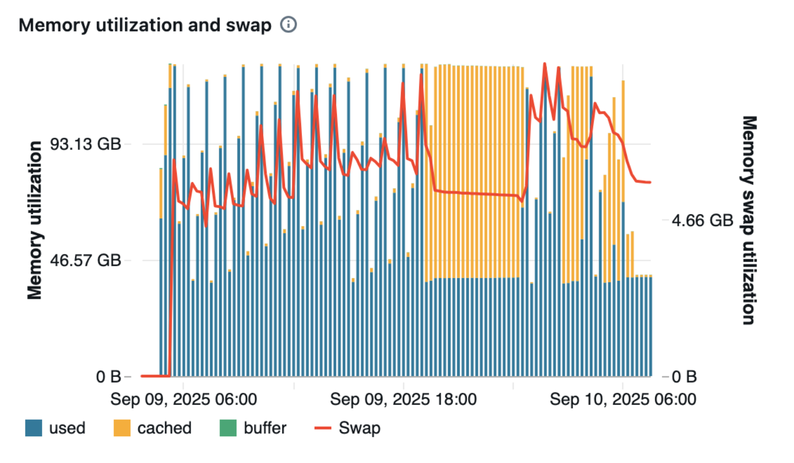
The cluster maintained memory utilization between 46-93 GB throughout the data transfer process, with very low swap usage. This indicates that the 128 GB RAM instance was sufficient to handle the PostgreSQL to Delta Lake data ingestion efficiently, with most data processing happening in memory rather than relying on disk-based swap.

2. Iceberg (Using OLake)

For the Iceberg path, we leveraged OLake, an open-source data replication tool specifically optimized for high-throughput data lake ingestion.

OLake’s Advantage:

• Delivers high throughput through parallelized data chunking, resumable historical snapshots, and lightning-fast incremental updates, ensuring exactly-once reliability even at massive scale.
• OLake’s setup is really simple and UI-driven, which made our data ingestion process much easier. Instead of spending time writing and optimizing code like in traditional ETL tools, we just configure everything through OLake’s intuitive interface which is extremely user friendly.

Important to Know!

In our runs, OLake was configured with max_threads=32 for ingestion parallelism.

• Memory Utilization
• CPU Usage

"system_memory_used_gb": {    "min": 4.023582458496094,    "max": 61.19172668457031,    "mean": 49.14759881837982,    "count": 8628}

• The system memory usage ranged from a minimum of 4.02 GB to a maximum of 61.19 GB, with an average of 49.15 GB throughout the transfer process. This indicates that the 128GB RAM instance was sufficient.
• We could have increased the parallel processing by increasing the number of threads, and still would have been within the 128GB RAM limit. The optimal memory usage has been observed here on the OLake’s side.

Comparing both the approaches:

When comparing our two data transfer approaches from local PostgreSQL to their destinations—Databricks Delta tables via a single-stream JDBC pipeline and Iceberg on S3 via a high‑throughput OLake pipeline—we observed clear differences in speed, operational effort, and cost, along with meaningful trade‑offs in reliability and flexibility.

Dimensions	Databricks	OLake
Transfer Time	25.7 hours	~12 hours
Transfer Cost	n2-standard-32($1.55/hr) = ~$39	Standard_D32s_v6 (32 vCPU, 64 GB RAM)($1.61/hr) = ~$20
Operational Comfort	Tedious	Extremely Simple

The transfer time clearly shows the difference—one method took around 25 hours, while the other finished in less than half that time.

Time and cost move together in data engineering—longer runs mean higher bills. OLake’s high throughput reduces runtime and, by extension, infrastructure cost. Plus, OLake is open source, so you’re only paying for the compute and storage you choose to provision.

The final question is comfort: How effortless is it for a data engineer to get from “connect” to “complete”?

On Databricks, we wrote extensive Python—managing source/target connections, selecting tables, and building a custom transfer pipeline—powerful, but undeniably tedious for bulk loads.

With OLake, the workflow was point‑and‑click: enter source and destination configs, select tables, hit Sync, and watch progress. It’s the kind of setup where you can watch a movie and eat pizza while the data moves—because that’s how easy it is!

C. Running TPCH queries​

With our 1TB dataset successfully loaded into both platforms, the real test begins. This is where architectural decisions, query optimization strategies, and compute orchestration converge into raw performance numbers. Over the course of our benchmark, we executed all 22 TPC-H queries sequentially on both platforms, measuring execution time down to the second.

Important benchmarking note: To keep the comparison apples-to-apples, we aimed to run the same Spark TPC-H code on both platforms. On the Iceberg side, we observed minor difficulties and adjusted accordingly:

With 64 shuffle partitions, we encountered memory pressure (OOM) and failures, so we set partitions to 128. 1.

We had to turn off vectorized reading due to an Arrow “Buffer index out of bounds” error (when processing certain Parquet pages with DOUBLE columns, the Arrow buffer allocation logic did not size the buffer correctly, creating a 0‑byte buffer when ~40KB was required). Because of this, we switched to non‑vectorized reading, which definitely affects the speed to query the data.

Code used to run the TPC-H queries for Databricks:

Show query runner code — Databricks

import timeimport logging# Setup logginglogging.basicConfig(level=logging.INFO, format='%(asctime)s - %(levelname)s - %(message)s')logger = logging.getLogger('tpch_benchmark')def configure_spark_settings():    """Configure Spark settings to optimize query execution"""    spark.conf.set("spark.sql.adaptive.enabled", "true")    spark.conf.set("spark.sql.adaptive.coalescePartitions.enabled", "true")    spark.conf.set("spark.sql.shuffle.partitions", "64")    logger.info("Spark configurations set: Adaptive Query Execution enabled, Coalesce Partitions enabled, shuffle partitions set to 64")def run_tpch_query(query_num, sql_query):    """Run a single TPC-H query with timing and logging"""    query_name = f"TPC-H Query {query_num}"    logger.info(f"Starting {query_name}")        start_time = time.perf_counter()    try:        # Execute the exact SQL query as provided        if query_num == 15 and isinstance(sql_query, list):            for i, sql_stmt in enumerate(sql_query):                logger.info(f"{query_name} - Executing statement {i+1}/3")                if i == 1:                    # SELECT statement: return/display results to force execution                    df = spark.sql(sql_stmt)                    df.show()                else:                    # CREATE VIEW and DROP VIEW statements                    spark.sql(sql_stmt)        else:            # All other queries are single-statement            df = spark.sql(sql_query)            df.show()                end_time = time.perf_counter()        execution_time = end_time - start_time                logger.info(f"{query_name} completed successfully in {execution_time:.2f} seconds")                return {            'query_number': query_num,            'time_seconds': execution_time,            'status': 'SUCCESS'        }                except Exception as e:        end_time = time.perf_counter()        execution_time = end_time - start_time        logger.error(f"{query_name} failed after {execution_time:.2f} seconds - Error: {str(e)}")                return {            'query_number': query_num,            'time_seconds': execution_time,            'status': 'FAILED',            'error': str(e)        }# All 22 TPC-H Queries exactly as provided in your filetpch_queries = {    1: """SELECTl_returnflag,l_linestatus,SUM(l_quantity) AS sum_qty,SUM(l_extendedprice) AS sum_base_price,SUM(l_extendedprice * (1 - l_discount)) AS sum_disc_price,SUM(l_extendedprice * (1 - l_discount) * (1 + l_tax)) AS sum_charge,AVG(l_quantity) AS avg_qty,AVG(l_extendedprice) AS avg_price,AVG(l_discount) AS avg_disc,COUNT(*) AS count_orderFROM datazip.testing3.lineitemWHERE l_shipdate <= DATE '1998-12-01' - INTERVAL '90' DAYGROUP BY l_returnflag, l_linestatusORDER BY l_returnflag, l_linestatus""",    2: """SELECTs_acctbal,s_name,n_name,p_partkey,p_mfgr,s_address,s_phone,s_commentFROMdatazip.testing3.part,datazip.testing3.supplier,datazip.testing3.partsupp,datazip.testing3.nation,datazip.testing3.regionWHEREp_partkey = ps_partkeyAND s_suppkey = ps_suppkeyAND p_size = 15AND p_type LIKE '%BRASS'AND s_nationkey = n_nationkeyAND n_regionkey = r_regionkeyAND r_name = 'EUROPE'AND ps_supplycost = (SELECT MIN(ps_supplycost)FROM datazip.testing3.partsupp, datazip.testing3.supplier, datazip.testing3.nation, datazip.testing3.regionWHERE p_partkey = ps_partkeyAND s_suppkey = ps_suppkeyAND s_nationkey = n_nationkeyAND n_regionkey = r_regionkeyAND r_name = 'EUROPE')ORDER BYs_acctbal DESC,n_name,s_name,p_partkeyLIMIT 100""",    3: """SELECTl_orderkey,SUM(l_extendedprice * (1 - l_discount)) AS revenue,o_orderdate,o_shippriorityFROMdatazip.testing3.customer,datazip.testing3.orders,datazip.testing3.lineitemWHEREc_mktsegment = 'BUILDING'AND c_custkey = o_custkeyAND l_orderkey = o_orderkeyAND o_orderdate < DATE '1995-03-15'AND l_shipdate > DATE '1995-03-15'GROUP BYl_orderkey,o_orderdate,o_shippriorityORDER BYrevenue DESC,o_orderdateLIMIT 10""",    4: """SELECTo_orderpriority,COUNT(*) AS order_countFROM datazip.testing3.ordersWHEREo_orderdate >= DATE '1993-07-01'AND o_orderdate < DATE '1993-07-01' + INTERVAL '3' MONTHAND EXISTS (SELECT *FROM datazip.testing3.lineitemWHERE l_orderkey = o_orderkeyAND l_commitdate < l_receiptdate)GROUP BY o_orderpriorityORDER BY o_orderpriority""",    5: """SELECTn_name,SUM(l_extendedprice * (1 - l_discount)) AS revenueFROMdatazip.testing3.customer,datazip.testing3.orders,datazip.testing3.lineitem,datazip.testing3.supplier,datazip.testing3.nation,datazip.testing3.regionWHEREc_custkey = o_custkeyAND l_orderkey = o_orderkeyAND l_suppkey = s_suppkeyAND c_nationkey = s_nationkeyAND s_nationkey = n_nationkeyAND n_regionkey = r_regionkeyAND r_name = 'ASIA'AND o_orderdate >= DATE '1994-01-01'AND o_orderdate < DATE '1994-01-01' + INTERVAL '1' YEARGROUP BY n_nameORDER BY revenue DESC""",    6: """SELECT SUM(l_extendedprice * l_discount) AS revenueFROM datazip.testing3.lineitemWHEREl_shipdate >= DATE '1994-01-01'AND l_shipdate < DATE '1994-01-01' + INTERVAL '1' YEARAND l_discount BETWEEN 0.06 - 0.01 AND 0.06 + 0.01AND l_quantity < 24""",    7: """SELECTsupp_nation,cust_nation,l_year,SUM(volume) AS revenueFROM (SELECTn1.n_name AS supp_nation,n2.n_name AS cust_nation,EXTRACT(YEAR FROM l_shipdate) AS l_year,l_extendedprice * (1 - l_discount) AS volumeFROMdatazip.testing3.supplier,datazip.testing3.lineitem,datazip.testing3.orders,datazip.testing3.customer,datazip.testing3.nation n1,datazip.testing3.nation n2WHEREs_suppkey = l_suppkeyAND o_orderkey = l_orderkeyAND c_custkey = o_custkeyAND s_nationkey = n1.n_nationkeyAND c_nationkey = n2.n_nationkeyAND ((n1.n_name = 'FRANCE' AND n2.n_name = 'GERMANY')OR (n1.n_name = 'GERMANY' AND n2.n_name = 'FRANCE'))AND l_shipdate BETWEEN DATE '1995-01-01' AND DATE '1996-12-31') AS shippingGROUP BY supp_nation, cust_nation, l_yearORDER BY supp_nation, cust_nation, l_year""",    8: """SELECTo_year,SUM(CASE WHEN nation = 'BRAZIL' THEN volume ELSE 0 END) / SUM(volume) AS mkt_shareFROM (SELECTEXTRACT(YEAR FROM o_orderdate) AS o_year,l_extendedprice * (1 - l_discount) AS volume,n2.n_name AS nationFROMdatazip.testing3.part,datazip.testing3.supplier,datazip.testing3.lineitem,datazip.testing3.orders,datazip.testing3.customer,datazip.testing3.nation n1,datazip.testing3.nation n2,datazip.testing3.regionWHEREp_partkey = l_partkeyAND s_suppkey = l_suppkeyAND l_orderkey = o_orderkeyAND o_custkey = c_custkeyAND c_nationkey = n1.n_nationkeyAND n1.n_regionkey = r_regionkeyAND r_name = 'AMERICA'AND s_nationkey = n2.n_nationkeyAND o_orderdate BETWEEN DATE '1995-01-01' AND DATE '1996-12-31'AND p_type = 'ECONOMY ANODIZED STEEL') AS all_nationsGROUP BY o_yearORDER BY o_year""",    9: """SELECTnation,o_year,SUM(amount) AS sum_profitFROM (SELECTn_name AS nation,EXTRACT(YEAR FROM o_orderdate) AS o_year,l_extendedprice * (1 - l_discount) - ps_supplycost * l_quantity AS amountFROMdatazip.testing3.part,datazip.testing3.supplier,datazip.testing3.lineitem,datazip.testing3.partsupp,datazip.testing3.orders,datazip.testing3.nationWHEREs_suppkey = l_suppkeyAND ps_suppkey = l_suppkeyAND ps_partkey = l_partkeyAND p_partkey = l_partkeyAND o_orderkey = l_orderkeyAND s_nationkey = n_nationkeyAND p_name LIKE '%green%') AS profitGROUP BY nation, o_yearORDER BY nation, o_year DESC""",    10: """SELECTc_custkey,c_name,SUM(l_extendedprice * (1 - l_discount)) AS revenue,c_acctbal,n_name,c_address,c_phone,c_commentFROMdatazip.testing3.customer,datazip.testing3.orders,datazip.testing3.lineitem,datazip.testing3.nationWHEREc_custkey = o_custkeyAND l_orderkey = o_orderkeyAND o_orderdate >= DATE '1993-10-01'AND o_orderdate < DATE '1993-10-01' + INTERVAL '3' MONTHAND l_returnflag = 'R'AND c_nationkey = n_nationkeyGROUP BYc_custkey,c_name,c_acctbal,c_phone,n_name,c_address,c_commentORDER BY revenue DESCLIMIT 20""",    11: """SELECTps_partkey,SUM(ps_supplycost * ps_availqty) AS valueFROMdatazip.testing3.partsupp,datazip.testing3.supplier,datazip.testing3.nationWHEREps_suppkey = s_suppkeyAND s_nationkey = n_nationkeyAND n_name = 'GERMANY'GROUP BY ps_partkeyHAVING SUM(ps_supplycost * ps_availqty) > (SELECT SUM(ps_supplycost * ps_availqty) * 0.0001FROMdatazip.testing3.partsupp,datazip.testing3.supplier,datazip.testing3.nationWHEREps_suppkey = s_suppkeyAND s_nationkey = n_nationkeyAND n_name = 'GERMANY')ORDER BY value DESC""",    12: """SELECTl_shipmode,SUM(CASEWHEN o_orderpriority = '1-URGENT'OR o_orderpriority = '2-HIGH'THEN 1ELSE 0END) AS high_line_count,SUM(CASEWHEN o_orderpriority <> '1-URGENT'AND o_orderpriority <> '2-HIGH'THEN 1ELSE 0END) AS low_line_countFROMdatazip.testing3.orders,datazip.testing3.lineitemWHEREo_orderkey = l_orderkeyAND l_shipmode IN ('MAIL', 'SHIP')AND l_commitdate < l_receiptdateAND l_shipdate < l_commitdateAND l_receiptdate >= DATE '1994-01-01'AND l_receiptdate < DATE '1994-01-01' + INTERVAL '1' YEARGROUP BY l_shipmodeORDER BY l_shipmode""",    13: """SELECTc_count,COUNT(*) AS custdistFROM (SELECTc_custkey,COUNT(o_orderkey) AS c_countFROMdatazip.testing3.customer LEFT OUTER JOIN datazip.testing3.orders ONc_custkey = o_custkeyAND o_comment NOT LIKE '%special%requests%'GROUP BY c_custkey) c_ordersGROUP BY c_countORDER BY custdist DESC, c_count DESC""",    14: """SELECT100.00 * SUM(CASEWHEN p_type LIKE 'PROMO%'THEN l_extendedprice * (1 - l_discount)ELSE 0END) / SUM(l_extendedprice * (1 - l_discount)) AS promo_revenueFROMdatazip.testing3.lineitem,datazip.testing3.partWHEREl_partkey = p_partkeyAND l_shipdate >= DATE '1995-09-01'AND l_shipdate < DATE '1995-09-01' + INTERVAL '1' MONTH""",    15: [        """CREATE OR REPLACE TEMPORARY VIEW revenue0 AS        SELECT          l_suppkey AS supplier_no,          SUM(l_extendedprice * (1 - l_discount)) AS total_revenue        FROM datazip.testing3.lineitem        WHERE          l_shipdate >= DATE '1996-01-01'          AND l_shipdate < DATE '1996-01-01' + INTERVAL '3' MONTH        GROUP BY l_suppkey""",        """SELECT          s_suppkey,          s_name,          s_address,          s_phone,          total_revenue        FROM          datazip.testing3.supplier,          revenue0        WHERE          s_suppkey = supplier_no          AND total_revenue = (            SELECT MAX(total_revenue) FROM revenue0          )        ORDER BY s_suppkey""",        """DROP VIEW revenue0"""    ],    16: """SELECTp_brand,p_type,p_size,COUNT(DISTINCT ps_suppkey) AS supplier_cntFROMdatazip.testing3.partsupp,datazip.testing3.partWHEREp_partkey = ps_partkeyAND p_brand <> 'Brand#45'AND p_type NOT LIKE 'MEDIUM POLISHED%'AND p_size IN (49, 14, 23, 45, 19, 3, 36, 9)AND ps_suppkey NOT IN (SELECT s_suppkeyFROM datazip.testing3.supplierWHERE s_comment LIKE '%Customer%Complaints%')GROUP BY p_brand, p_type, p_sizeORDER BY supplier_cnt DESC, p_brand, p_type, p_size""",    17: """SELECT SUM(l_extendedprice) / 7.0 AS avg_yearlyFROMdatazip.testing3.lineitem,datazip.testing3.partWHEREp_partkey = l_partkeyAND p_brand =