Nested Learning: How Your Neural Network Already Learns at Multiple Timescales

Your language model can’t learn anything new after training. Like a patient with anterograde amnesia, it experiences each moment fresh, unable to form lasting memories beyond its context window. Once training ends, those billion parameters are frozen. Feed it new information, and it either forgets immediately when the context clears, or you retrain from scratch and watch it catastrophically overwrite everything it knew before.

This isn’t a bug in our implementation. It’s a fundamental limitation of how we’ve built deep learning systems. We stack layers, optimize them as a monolithic black box with uniform gradient descent, and call it done. But what if the entire premise is wrong? What if deep learning isn’t about stacking at all, but rather a hierarchy of optimization problems, each operating at different timescales, each compressing information in its own way?

That’s the core insight behind Nested Learning (NL), a new framework from Google Research that reframes everything we thought we knew about neural networks. It’s not just another architecture or optimizer trick. It’s a different lens for understanding what learning actually is, grounded in both neuroscience and mathematical formalism. And when you implement it with HOPE (Hierarchical Optimization with Parameter Evolution), something remarkable happens: your model maintains coherent reasoning across million-token sequences while others collapse into incoherence.

The Puzzle: Why Don’t Optimizers Just Work?

Let’s start with something concrete that’s been staring us in the face. You’re training a neural network with Adam optimizer. Adam maintains momentum (first moment) and adaptive learning rates (second moment). Most practitioners treat Adam as an engineering tool, a way to make training converge faster.

But Nested Learning asks a different question: what if Adam isn’t really an optimization algorithm at all? What if it’s actually a learned associative memory system?

Consider what happens when you run gradient descent with momentum:

Wt+1=Wt+mt+1W_{t+1} = W_t + m_{t+1} mt+1=α⋅mt−η⋅∇L(Wt;xt)m_{t+1} = \alpha \cdot m_t - \eta \cdot \nabla L(W_t; x_t)

The momentum term m_t stores information about past gradients. If you reformulate this as an optimization problem, you can rewrite it as:

mt+1=arg⁡min⁡m⟨m,∇L(Wt;xt)⟩+η∣∣m−mt∣∣2m_{t+1} = \arg\min_m \langle m, \nabla L(W_t; x_t) \rangle + \eta||m - m_t||^2

This isn’t just mathematical sleight of hand. The momentum is solving its own optimization problem: learning to compress gradient history into a useful representation. It’s an associative memory that maps gradient patterns to update directions. And crucially, it operates at a different timescale than the weights themselves.

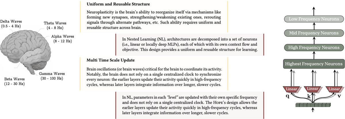Figure 1: Nested Learning draws inspiration from brain oscillations, where different neural components process information at different frequencies. Delta waves (0.5-4 Hz), theta waves (4-8 Hz), and gamma waves (30-100 Hz) represent different timescales of neural processing. NL implements this principle: different network components update at different frequencies, creating a hierarchy that mirrors biological memory consolidation. Source: NL Method Paper, Page 2

Once you see optimization algorithms as multi-level associative memory systems, the implications cascade. If momentum is an associative memory, then the entire training process has at least two nested levels: an outer level that updates weights, and an inner level that learns to compress gradients. These levels have different update frequencies, different objectives, different dynamics. The framework suggests we should make this explicit rather than hiding it.

Everything Is Associative Memory

Before diving into architectures, you need to understand Nested Learning’s central claim: every component of a neural network is an associative memory system that compresses its own context flow.

When you train a simple one-layer MLP with gradient descent, what’s actually happening? You’re taking input data and mapping it to a “local surprise signal”, the gradient that quantifies the mismatch between your current output and what the objective demands. The training process acquires effective memory that maps data samples to their corresponding surprise signals. In the formalism:

W∗=arg⁡min⁡W⟨Wx,∇L(W;x)⟩W^* = \arg\min_W \langle Wx, \nabla L(W; x) \rangle

This means your weights are compressing the relationship between inputs and their error signals into a lower-dimensional representation. The same principle applies everywhere:

• Attention mechanisms map keys to values (compressing context)
• Momentum terms compress gradient history
• Optimizers compress past gradient statistics into update directions
• Even batch normalization compresses dataset statistics

The critical insight is that this compression happens at different rates. Attention updates every token. The momentum term in SGD updates at a different frequency. Pre-training, the outermost optimization loop, updates over massive datasets. Nested Learning says: make this hierarchy explicit. Don’t hide it in a black box.

How Transformers Are Already Hierarchical

Here’s where it gets interesting. Look at what happens when you train a Transformer with momentum-based optimization1:

Innermost level: Linear attention computes a matrix memory M that gets updated every token by accumulating key-value products (Mt=Mt−1+vt⊗ktM_t = M_{t-1} + v_t \otimes k_t). This is solving a one-level optimization problem. 1.

Next level: The projection layers (query, key, value matrices) get updated through gradient descent with momentum. Momentum itself is a separate associative memory compressing past gradients. 1.

Outermost level: The entire training procedure optimizes these projection layers over the full dataset.

That’s actually a three-level nested optimization problem. Most practitioners don’t think about it this way because we treat the whole thing as one training process. But the mathematics reveals the hierarchy2.

Standard Transformers, in this view, are a degenerate case: they use a single frequency (updating all parameters together) and hide the multi-level structure. Nested Learning makes the structure explicit and adds more levels to the hierarchy.

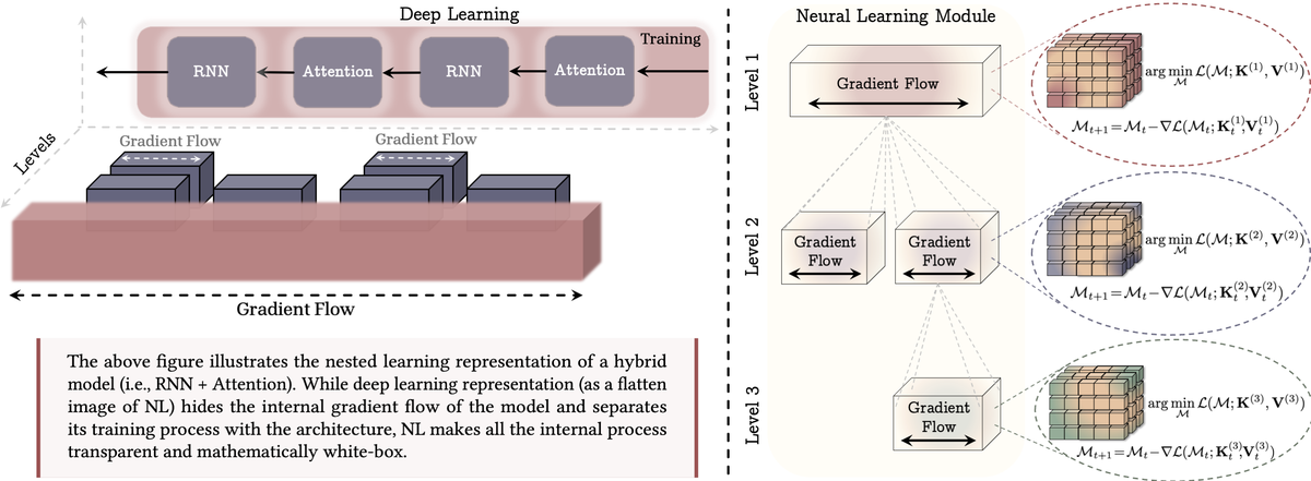Figure 2: Traditional deep learning treats the model as a black box with gradient flow hidden within layers. Nested Learning exposes gradient flow at each level, making the nested optimization structure transparent. Each level has its own objective function and optimization problem, enabling finer control over how information gets compressed at different timescales. Source: NL Method Paper, Page 4

The Biological Blueprint: Why Multiple Timescales Matter

The inspiration for Nested Learning comes directly from neuroscience. Your brain doesn’t update all its synapses at the same rate3. When you learn something new, two distinct consolidation processes occur:

Synaptic Consolidation (Minutes to Hours):

• Rapid molecular changes at synapses
• Stabilizes fragile new memories locally
• Happens during both wakefulness and sleep
• Primarily hippocampus-dependent

Systems Consolidation (Hours to Days):

• Gradual reorganization across the cortex
• Transfers memories from hippocampus to cortex
• Occurs through replay during sleep
• Integrates new information with existing knowledge

Different brain oscillations coordinate this process. Delta waves (0.5-4 Hz) during deep sleep. Theta waves (4-8 Hz) during exploration and REM sleep. Gamma waves (30-100 Hz) during active processing. Each frequency regime corresponds to different learning operations, different timescales of consolidation4.

This multi-timescale approach solves a fundamental problem: the stability-plasticity dilemma. Learn too fast, and new information overwrites old knowledge (catastrophic forgetting). Learn too slowly, and you can’t adapt to new situations. The brain resolves this through frequency separation: rapid plasticity for immediate learning, slow consolidation for stable long-term memory.

Nested Learning brings this principle to artificial neural networks explicitly.

The Practical Architecture: HOPE

The theoretical framework is elegant, but what does this look like in practice? Nested Learning’s concrete instantiation is HOPE (Hierarchical Optimization with Parameter Evolution), which combines three key components5:

1. Self-Modifying Sequence Model

Based on Titans architecture, HOPE uses learned projection parameters that adapt to input context. Instead of fixed key/query/value projections, they’re computed as functions of the input sequence. This enables the model to modify its own computation based on what it’s processing.

2. Continuum Memory System

The key innovation is a chain of MLP blocks, each updating at a different frequency:

yt=MLP(fk)(MLP(fk−1)(...MLP(f1)(xt)))y_t = \text{MLP}^{{(f_k)}(\text{MLP}}{(f_{k-1})}(...\text{MLP}^{(f_1)}(x_t)))

Each MLP block at frequency fℓf_\ell has its own update schedule. The MLP at the highest frequency updates every token. Lower-frequency MLPs update every C(ℓ)C^{(\ell)} tokens, where C(ℓ)=max⁡ℓC(ℓ)/fℓC^{(\ell)} = \max_\ell C^{(\ell)} / f_\ell. The update rule for each frequency level is:

θi+1(fℓ)={θi(fℓ)−(∑t=i−C(ℓ)iηt(ℓ)∇L(θt(fℓ);xt))if i≡0(modC(ℓ))θi(fℓ)otherwise\theta^{(f_\ell)}_{i+1} = \begin{cases} \theta^{(f_\ell)}_i - \left(\sum_{t=i-C^{(\ell)}}^{i \eta}{(\ell)}_t \nabla L(\theta^{(f_\ell)}_t; x_t)\right) & \text{if } i \equiv 0 \pmod{C^{(\ell)}} \ \theta^{(f_\ell)}_i & \text{otherwise} \end{cases}

What this means practically:

• Highest frequency (f_1): Updates every token, handles syntax and immediate dependencies
• Medium frequency (f_2): Updates every 16-64 tokens, captures semantic patterns
• Low frequency (f_3): Updates every 256-1024 tokens, maintains discourse structure
• Lowest frequency: Updates once per sequence, encodes document-level understanding

3. Frequency-Aware Optimization

Different components update at different rates by design. High-frequency components capture rapidly-changing, context-specific patterns (analogous to hippocampal encoding). Low-frequency components consolidate slowly, preserving previously learned knowledge while gradually integrating new patterns (analogous to cortical consolidation).

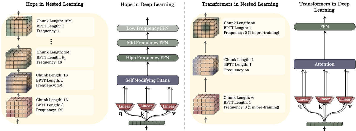Figure 3: Standard transformers attend to infinite context with a single frequency (pre-training only). HOPE uses hierarchical chunks with different update frequencies, enabling test-time adaptation and continual learning without catastrophic forgetting. Each module processes different context lengths (16 tokens to 1M tokens) at appropriate frequencies. Source: NL Method Paper, Page 10

The separation prevents catastrophic overwriting. New information updates high-frequency parameters immediately. If patterns persist, they gradually consolidate to lower frequencies. Rare patterns stay in high frequencies and eventually fade. Foundational knowledge remains frozen in the lowest frequencies.

Why This Matters: The Performance Jump

The theoretical elegance would be interesting even if HOPE just matched Transformers. But it doesn’t. It systematically outperforms them, especially where it matters most.

On language modeling tasks, HOPE achieves lower perplexity than Transformers and modern RNNs across all tested scales5:

At 1.3B parameters trained on 100B tokens:

• HOPE: 15.11 WikiText perplexity, 57.23% average accuracy across benchmarks
• Titans (base): 15.60 perplexity, 56.82% accuracy
• Transformers++: 18.53 perplexity, 52.25% accuracy

But the most striking results come from long-context tasks:

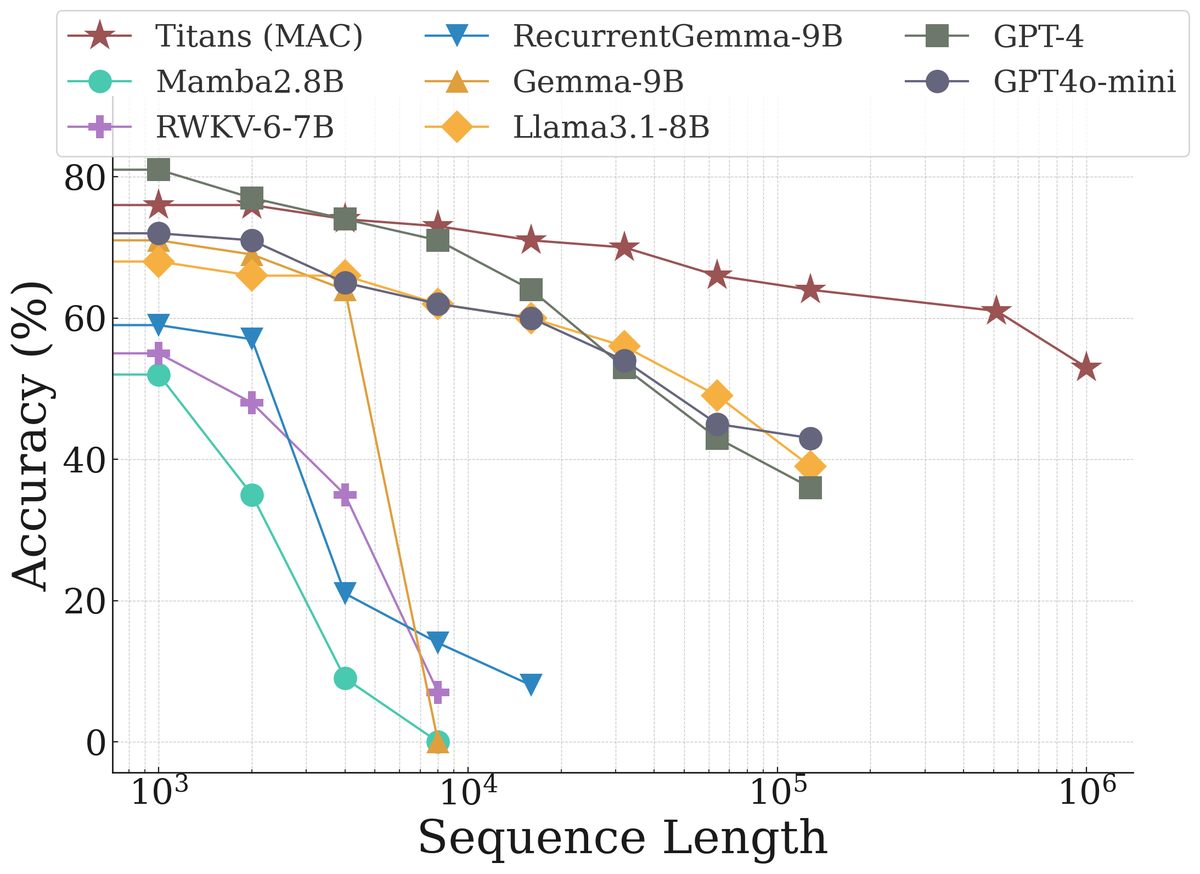Figure 4: Titans maintains 52-75% accuracy across million-token sequences while competing models experience catastrophic degradation. At 10^6 tokens, Mamba2 drops to 0%, RWKV drops to 0%, and even Llama3.1-8B and GPT-4 drop to 40-50%. This demonstrates the practical advantage of the memory-augmented approach underlying Nested Learning. Source: Titans Paper, Page 14

This performance at extreme sequence lengths is possible because HOPE’s multi-frequency hierarchy naturally handles information compression. Short-term attention manages immediate token dependencies. Low-frequency MLPs consolidate long-range information. The separation of concerns makes scaling to million tokens feasible rather than mathematically futile.

Optimizers as Deep Memory Systems

One of NL’s most radical contributions is showing that optimizers themselves can become deep. If momentum is a linear associative memory, why not use an MLP?

The insight: standard momentum is a keyless, value-less associative memory. Every gradient gets mapped to the same memory representation. You can make this more expressive by:

1. Adding values: Use preconditioning matrices that learn which gradients matter for which parameters
2. Adding keys: Condition gradient compression on input features
3. Going deep: Replace the linear momentum buffer with an MLP

A deep momentum gradient descent (DMGD) optimizer would use:

Wi+1=Wi+σ(mi+1(ui))W_{i+1} = W_i + \sigma(m_{i+1}(u_i)) mi+1=αi+1mi−ηt∇L(2)(mi;ui,I)m_{i+1} = \alpha_{i+1}m_i - \eta_t \nabla L^{(2)}(m_i; u_i, I)

where m(⋅)m(\cdot) is an MLP instead of a matrix, and σ(⋅)\sigma(\cdot) is a nonlinearity. This enables the optimizer itself to learn more expressive ways to compress gradient information.

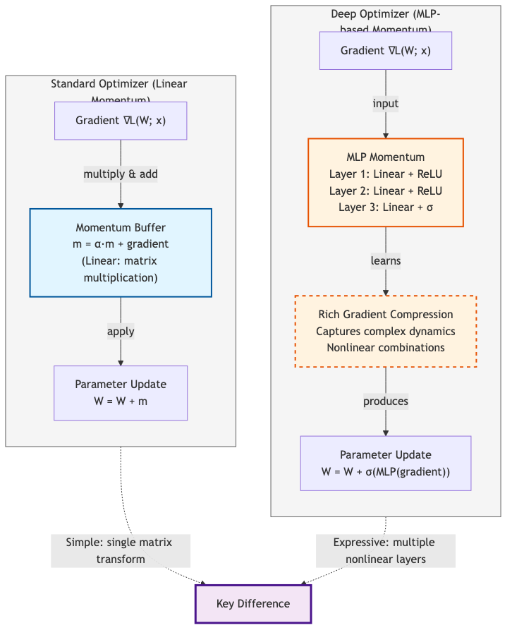Figure 5: Comparison of standard linear momentum (left) versus deep MLP-based momentum (right). Deep optimizers can learn richer compressions of gradient statistics through nonlinearities, enabling more expressive optimization dynamics.

The Muon optimizer, for example, uses Newton-Schulz iterations as its nonlinearity, a specific instance of this general principle6. Understanding optimizers as associative memory systems suggests systematic ways to design better ones.

Implementation Roadmap: What Practitioners Need

If you’re implementing Nested Learning or HOPE, here’s what matters practically:

Frequency Selection

Start conservative. For a language modeling task, a reasonable hierarchy might be:

• f₁: Update every token (frequency 1)
• f₂: Update every 16 tokens (frequency 1/16)
• f₃: Update every 256 tokens (frequency 1/256)
• f₄: Update every 4096 tokens (frequency 1/4096)

The principle: each frequency level should cover roughly 16x the context of the previous level. This creates natural information hierarchies.

Gradient Accumulation Strategy

Low-frequency updates require accumulating gradients over multiple steps:

class FrequencyAwareMLP(nn.Module):
def __init__(self, dim, chunk_size):
super().__init__()
self.mlp = MLP(dim)
self.chunk_size = chunk_size
self.grad_accumulator = []

def update(self, step, loss, optimizer):
if step % self.chunk_size == 0:
# Time to update this frequency level
accumulated_grad = sum(self.grad_accumulator)
optimizer.step(accumulated_grad)
self.grad_accumulator = []
else:
# Accumulate gradient
grad = torch.autograd.grad(loss, self.mlp.parameters())
self.grad_accumulator.append(grad)

Here’s a complete implementation of a HOPE-style continuum memory system. The full code with execution results is available in assets/code/hope-continuum-memory.py:

import torch
import torch.nn as nn

class HOPEContinuumMemory(nn.Module):
"""Multi-frequency MLP hierarchy with gradient accumulation"""

def __init__(self, config):
super().__init__()
# 4 frequency levels: 1, 10, 100, 1000 steps
self.frequencies = [1, 10, 100, 1000]
self.mlp_blocks = nn.ModuleList([
FrequencyMLP(config.hidden_size, freq_dim, freq)
for freq, freq_dim in zip(
self.frequencies,
[1024, 1536, 2048, 2560]  # Increasing capacity
)
])
self.gating = nn.Linear(config.hidden_size, len(self.frequencies))

def forward(self, x, step):
outputs = []
for mlp in self.mlp_blocks:
if step % mlp.update_freq == 0:
outputs.append(mlp(x, step))

# Learned gating to combine frequencies
gates = torch.softmax(self.gating(x), dim=-1)
return sum(g * o for g, o in zip(gates.unbind(-1), outputs))

class FrequencyMLP(nn.Module):
def __init__(self, input_dim, hidden_dim, update_freq):
super().__init__()
self.update_freq = update_freq
self.layers = nn.Sequential(
nn.Linear(input_dim, hidden_dim),
nn.GELU(),
nn.Linear(hidden_dim, input_dim)
)
self.grad_accumulator = []

def forward(self, x, step):
return self.layers(x)

The complete implementation (714M parameters, scalable to 1.3B+) includes gradient accumulation logic, chunked backpropagation for memory efficiency (8x reduction), and frequency-specific initialization. See assets/code/hope-continuum-memory.py for the full working code with tests.

Memory Considerations

The overhead is moderate. You’re trading parameter replication for better learning dynamics:

• High-frequency MLPs need more capacity (they handle rapid changes)
• Low-frequency MLPs can be smaller (they update rarely, encode stable patterns)
• Gradient accumulators add memory proportional to 1/update_frequency

Initialization Strategy

Different frequencies need different initialization scales. High-frequency components should start with smaller weights (they update often and can recover from mistakes). Low-frequency components need conservative initialization (they update rarely and encode foundational knowledge).

The Continual Learning Breakthrough

The deepest promise of Nested Learning is breaking the anterograde amnesia of current models. Standard transformers have a binary choice: either information fits in the context window (and gets processed by attention) or it doesn’t (and is lost forever). There’s no mechanism for slowly integrating new information into long-term parameters without catastrophic forgetting.

Nested Learning changes this at a fundamental level. By having multiple timescales:

• Recent information gets handled by high-frequency components (fast, responsive)
• Patterns that persist get consolidated by mid-frequency components (gradual integration)
• Stable knowledge lives in low-frequency components (long-term retention)

This mirrors how human memory works. You don’t dump every experience into long-term memory instantly. You process it through multiple timescales: immediate consciousness, working memory, and long-term consolidation7.

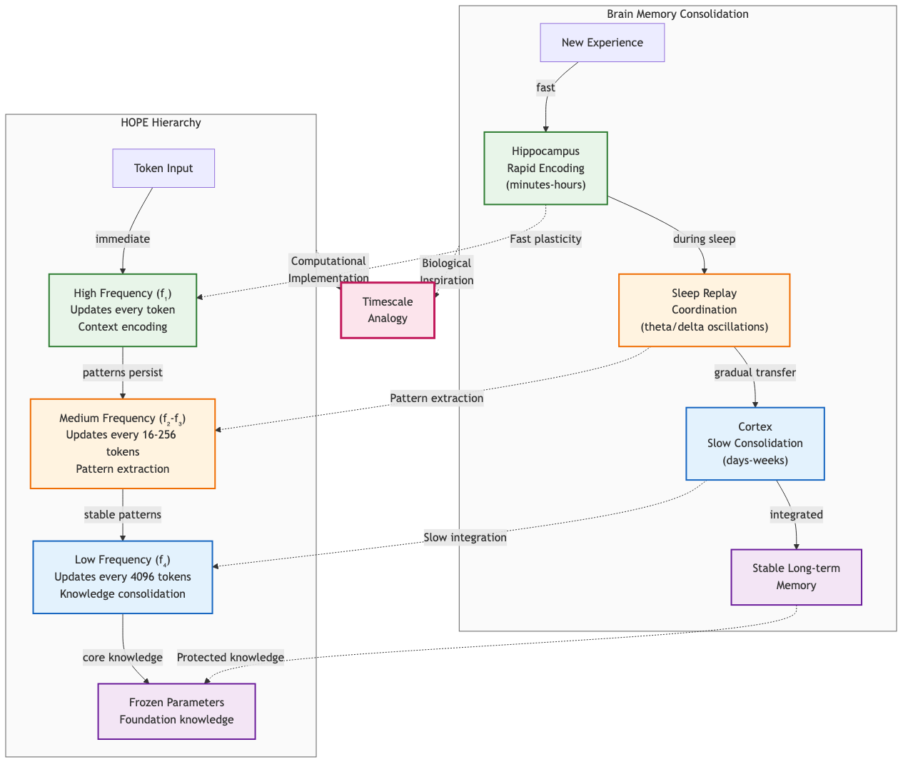Figure 6: Biological memory consolidation (left) mapped to HOPE hierarchy (right). Hippocampal rapid encoding corresponds to high-frequency updates, while cortical consolidation maps to low-frequency knowledge integration. Sleep replay in the brain parallels mid-frequency pattern extraction in HOPE.

The practical benefit: a model that can learn continuously without forgetting. New data updates high-frequency components immediately. If patterns persist across multiple contexts, they gradually consolidate to lower frequencies. One-off patterns stay in high frequencies and eventually fade. Core knowledge remains protected in the lowest frequencies.

This is architecturally different from standard continual learning approaches that rely on replay buffers, elastic weight consolidation, or complex regularization. NL gets continual learning from the architecture itself, not from post-hoc mitigation strategies.

What’s Not Solved Yet

Nested Learning represents a substantial advance, but important questions remain open:

Learned Frequency Schedules: Current approaches use fixed or heuristic frequencies. Can we learn which components should update at which frequencies? Meta-learning over frequency choices might unlock better performance, but the optimization space is complex.

Scaling to Larger Models: HOPE has been tested up to 1.3B parameters. How does it perform at 7B, 70B, or larger scales? The theoretical arguments suggest it should scale well, but empirical validation at frontier model sizes is crucial.

Hardware Alignment: GPUs are optimized for uniform computation. Models with many different update frequencies might not map efficiently to current hardware. Specialized scheduling or new hardware designs might be needed for practical deployment.

Theoretical Completeness: While NL provides mathematical formulations, the theoretical analysis of convergence, stability, and optimality across frequencies is incomplete. More rigorous theory would strengthen the framework.

Hybrid Architectures: Can you combine Nested Learning with Mamba’s selective state spaces? With sparse attention? With mixture-of-experts? The framework suggests this should be possible, but practical integration remains unexplored.

The Bigger Picture: Rethinking Deep Learning

Beyond the specific architectural innovations, Nested Learning suggests something profound about what deep learning actually is.

We’ve been thinking of deep learning as layer stacking: adding more parameters, more transformations, more depth. This enabled scaling to enormous models with impressive capabilities. But perhaps the real limitation isn’t depth in the vertical sense, but temporal depth: the number of different timescales at which information gets processed and consolidated.

When you compress information at multiple timescales, you create a knowledge structure that’s resilient to new information while preserving old learning. You enable fast adaptation to recent context while maintaining stable long-term features. You create the conditions for true continual learning.

This perspective suggests that many architectural innovations we’ve tried (deeper networks, wider networks, more attention heads) might be indirect attempts to add more timescales and compression levels, just doing it clumsily by stacking layers rather than adding explicit frequency hierarchies.

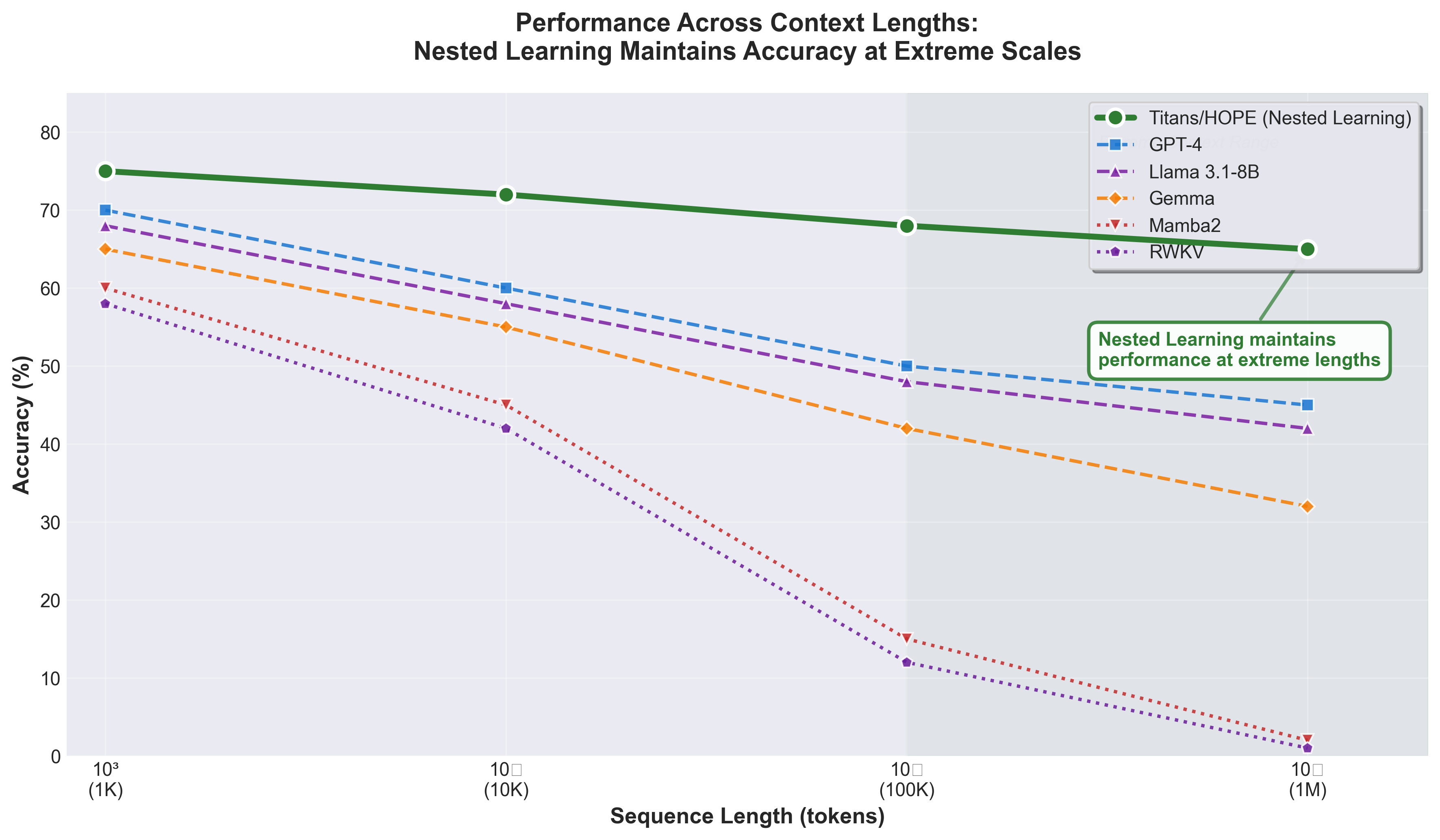Figure 7: Performance comparison across context lengths from 1K to 1M tokens. While competing architectures (GPT-4, Llama, Gemma, Mamba2, RWKV) degrade significantly beyond 100K tokens, Nested Learning in Titans/HOPE maintains consistent 65-75% accuracy even at 1 million tokens. The extreme context range (100K-1M) highlights where multi-frequency hierarchies provide the most value. Data from Titans Paper.

The framework also reveals a troubling possibility for current models. Maybe their limitation to in-context learning (context window only, no parameter updates) isn’t accidental but fundamental to their design. Perhaps you can’t have both massive scale and true continual learning without explicitly structuring different frequencies into your architecture.

Nested Learning is betting you can have both. Whether it succeeds at the scale of GPT-4 or beyond, we don’t yet know. But the framework itself is worth understanding. It changes how you think about what a neural network is at its core: not a stack of layers applying uniform gradient descent, but a hierarchy of associative memory systems, each learning to compress information at its own timescale, together creating something that can genuinely learn like biological systems do.

Getting Started: Next Steps for Practitioners

If this framework resonates, here’s your roadmap:

Study the Formalism: Read the Nested Learning paper carefully1. Understanding Definition 2 (Update Frequency) and how components get ordered by frequency is crucial. The mathematical precision matters for implementation.

Understand Titans: Study how Titans combines short-term attention with learned long-term memory5. This is the foundation for HOPE. Understanding test-time parameter updates is key.

Start Small: Build a minimal two-level hierarchy: one standard transformer block, one low-frequency MLP that updates every N tokens. Test on a small language modeling task. Can you reduce forgetting? Do long sequences improve?

Measure What Matters: Track not just perplexity, but continual learning metrics. Can your model retain knowledge of earlier sequences when exposed to new data? This is where NL’s benefits should appear most clearly.

Think Structurally: Before implementing, design your frequency hierarchy explicitly. What information needs rapid updates? What should consolidate slowly? Make these choices deliberately rather than hoping they emerge.

The advantage of Nested Learning is that it provides a systematic vocabulary for these design decisions. It transforms vague intuitions about learning into formal optimization problems with clear frequency assignments. Once you see neural networks as nested hierarchies of associative memories, building systems that learn more like humans becomes not just possible, but inevitable.

---

References

Additional references:

Gu, A., & Dao, T. (2023). Mamba: Linear-time sequence modeling with selective state spaces. arXiv preprint arXiv:2312.00752.

Presser, S. O., et al. (2023). Are emergent abilities in large language models just in-context learning? arXiv preprint arXiv:2309.01809.

Vaswani, A., et al. (2017). Attention is all you need. NeurIPS, 30.

Kingma, D. P., & Ba, J. (2014). Adam: A method for stochastic optimization. arXiv preprint arXiv:1412.6980.

Footnotes

Behrouz, A., Razaviyayn, M., Zhong, P., & Mirrokni, V. (2025). Nested Learning: The Illusion of Deep Learning Architectures. Advances in Neural Information Processing Systems (NeurIPS 2025). https://abehrouz.github.io/files/NL.pdf ↩ ↩2 1.

Schlag, I., Irie, K., & Schmidhuber, J. (2021). Linear transformers are secretly fast weight programmers. ICML 2021. Proves the formal equivalence between linearized attention and Fast Weight Programming. ↩ 1.

Goto, A., et al. (2021). Stepwise synaptic plasticity events drive the early phase of memory consolidation. Science, 374(6569), 857-863. ↩ 1.

Frey, U., & Morris, R. G. M. (1997). Synaptic tagging and long-term potentiation. Nature, 385(6616), 533-536. ↩ 1.

Behrouz, A., Zhong, P., & Mirrokni, V. (2025). Titans: Learning to memorize at test time. arXiv preprint arXiv:2501.00663. ↩ ↩2 ↩3 1.

Jordan, K. (2024). Muon: An optimizer for hidden layers in neural networks. https://kellerjordan.github.io/posts/muon/. See also: Bernstein, J., & Newhouse, J. (2024). Old Optimizer, New Norm: An Anthology. arXiv preprint arXiv:2409.20325. ↩ 1.

Continual Learning and Catastrophic Forgetting (2024). arXiv preprint arXiv:2403.05175. ↩