In the latest 0.3.0 release of Turso database we made several notable improvements for vector search support for both dense and sparse vectors: For dense vectors, we have introduced SIMD acceleration, allowing for faster exact search for dense operations. For sparse vectors, we have added a new, more efficient storage representation, and specialized indexing methods, allowing for a better approximate search.

In this post, we’ll dive deep into the sparse vectors indexing feature, which allows quick search for nearest neighbors by Weighted Jaccard distance in the collection of sparse vectors. We will show specializing for sparse vectors allow for a 5-50x space savings over dense vectors, and how the new indexing method delivers and an additional 21% speedup for approximate search.

#Sparse vectors and Jaccard distance

Vector search has exploded in popularity recently, on the back of the rise of LLMs. The vectors used by embedding models are dense vectors: most of its dimensions have some value. However, in more traditional machine learning domains, sparse vectors are still found. They remain a valuable tool in the domains like bioinformatics, text mining, computer vision and others.

Sparse vectors excel at comparing weighted feature sets. For example, you can measure document similarity by representing each document as a sparse vector, where each dimension is a dictionary word weighted by its tf-idf scores. Another example can be estimating genomes similarity by representing them as a sketch vector of k-mers.

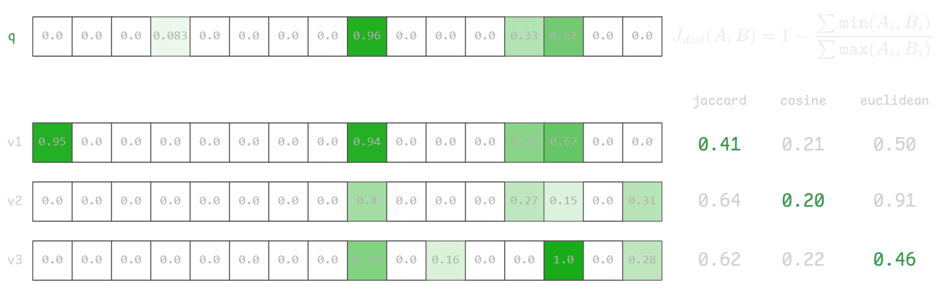
For these use cases, weighted Jaccard distance is the natural metric. Unlike cosine or Euclidean distance, which introduce artifacts from the underlying metric space geometry, Jaccard distance directly captures what matters: the overlap between weighted feature sets.

Consider an example below, where first vector v1 is the closest to q by Jaccard distance and clearly has good overlap with 3 features, but in cosine and Euclidian space this vector is worse than vectors v2 and v3.

#Index Methods in Turso

Starting with Turso 0.3.0 release, a vector can be stored usign the vector32_sparse function, as opposed to the general purpose vector32. Check the full documentation for more functions and examples. When only a small fraction of components are non-zero, sparse representation can use 5–50× less storage, meaning the search can check more vectors in a single database page. This alone leads to faster search: for sparse vectors, our benchmarks indicate that we can search upwards of 100k vectors in under 100 millisecods.

In order to make search even faster for larger datasets we need to add indexing. SQLite has a very flexible VTable concept which allows developers to hook into special SQL syntax and implement arbitrary data access logic under the hood.

The main VTable limitation is that it isn’t integrated into the query planner and needs to be maintained separately from the main table with the data. This leads to duplicate work for developers and more complex queries for users.

Being able to make deeper changes to SQLite was the whole point of starting the Turso project. To properly support vector indexes with great DX, we have introduced the Index Method feature. It allows database developers, including extension developers, to implement custom data access methods and neatly integrate them into the query planner.

For modification operations, Index Method integrates into the query planner similarly to native B-Tree indices. For query operations, every Index Method provides a set of patterns indicating where the index should be used. For example, in our case the query pattern will be like that:

SELECT vector_distance_jaccard({table_name}, ?) as distance
FROM {table_name}
ORDER BY distance
LIMIT ?

Note that each pattern defines multiple aspects with a single familiar SQL query:

1. Query pattern defines the output shape of the Index Method results
2. Query pattern defines parameters necessary for Index Method execution
3. Query pattern defines a “shape” of the query (or subquery) which can be optimized and replaced by Index Method by the engine

With this infrastructure in place, we can implement custom indexes for sparse vectors that neatly integrate into the database query planner.

#Sparse vectors index implementation

To build an efficient search index, we leverage the key property of sparse vectors: most components are zero.

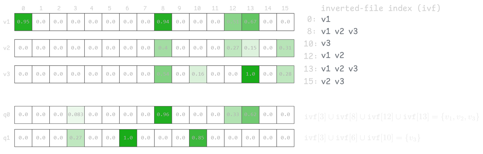
We can view our vector dataset as a collection of (rowid, component) pairs. A straightforward approach is to build an Inverted Index that efficiently retrieves all rows with non-zero values for a given component. To do that we store an ordered collection of (component, rowid) pairs, making it easy to enumerate all rows for any component.

This lets us calculate distance only for rows that share at least one non-zero component with the query vector, greatly reducing the search space when intersection is small.

In the example below, the inverted index allows us to calculate distance for only one row for query vector q1, since no other rows intersect with the query.

#Frequency-based Component Selection

Building the inverted index itself can already provide some speedup. But at the extreme, when a component can be present in a large portion of dataset (like common word in a text indexing case), we still need to enumerate all rows in the database and there will be no speedup for the search.

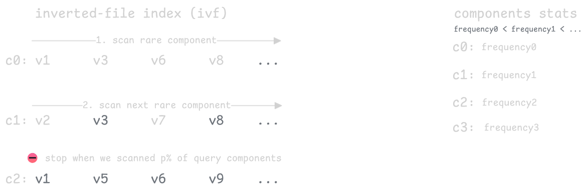
The key insight is that rare components are much more informative than common ones. Rare components are like unique keywords, they only appear in a few vectors, so vectors that share them are more likely to be similar. Common components tell us little since they’re everywhere.

We can exploit this by ranking the query’s components by how rare they are, then keeping only the rarest p%. We only calculate distances for vectors that match these rare components, which dramatically shrinks the search space. The parameter p lets you balance speed versus accuracy.

The tradeoff is that while this controls search size well, quality becomes unpredictable. Filtering out common components can miss relevant vectors that don’t happen to share the selected rare ones with your query, causing recall to vary significantly between queries.

#Adaptive Length Filtering

Since sparse vectors used for Jaccard distance always have non-negative weights, we can rewrite the distance formula to depend only on summed minimums and pre-computed vector totals.

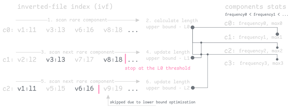
This reformulation enables a key optimization: as we process components (in reverse frequency order), we can estimate the maximum vector length that could possibly achieve a distance better than our current worst top-K result. When we find better candidates, we tighten this length threshold, eliminating vectors that can’t make the top-K.

The index stores (component, length, rowid) triplets plus component statistics (frequency and max value), allowing us to skip vectors above the length threshold for each component.

This approach includes a tuning parameter Δ that provides predictable guarantees. By relaxing the target distance to J + Δ, the index searches more aggressively while ensuring results differ from the optimal by at most Δ. Unlike frequency-based filtering, this gives you a bounded approximation—search quality is controllable and predictable

#Benchmarks

We evaluated the index and brute-force approaches on 400,000 embeddings for Amazon Reviews dataset where every sparse vector has 249,519 dimensions and 50 non-zero components on average (the embeddings were generated with default TfidfVectorizer()). Note that the default TfidfVectorizer uses a simple strategy for tokenization and does not stem words. So the vectorization process could be improved independently to get more relevant search results and improve performance. However, since we’re interested in pure vector search performance, we decided to keep the default settings for vectorizer.

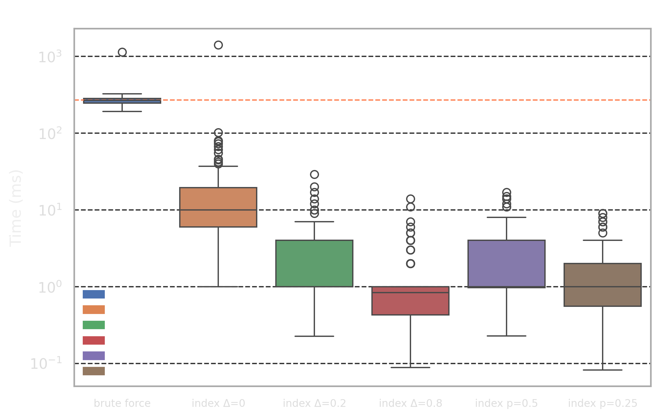
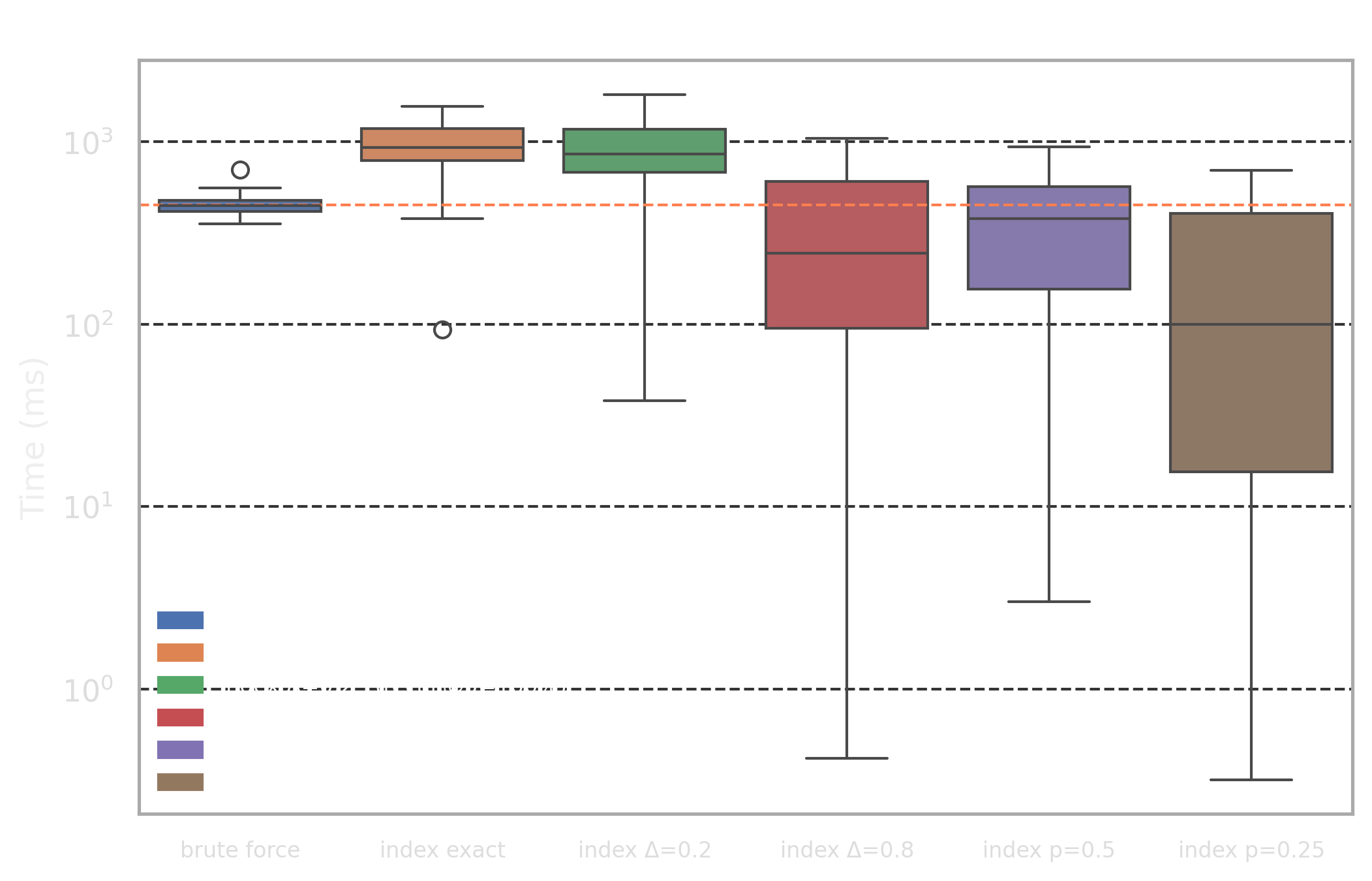
To benchmark the search we picked two different “profiles”:

1. High selectivity profile: for 100 randomly chosen reviews (50-200 words) we are trying to find 5 nearest documents by Jaccard distance
2. Low selectivity profile: for 100 randomly chosen search queries (3-8 words) we are trying to find 5 nearest documents by Jaccard distance

The difference between the profiles is that the “high selectivity profile” has many more components in the query vector compared to “low selectivity profile” and also has some portion of common words (this, then, etc) which will affect our optimizations.

We picked 6 different targets for the benchmark:

• brute force: naive approach without index where the distance is calculated for every row
• index exact: exact index with length optimization Δ=0.0
• Approximate indices with adaptive length optimization for Δ=0.2/Δ=0.8
• Approximate indices with component selection optimization which uses only the p=50%/p=25% rarest components from the query vector

To evaluate the quality of the approximate indices, we use the recall@5 metric, which measures the proportion of the true top-5 nearest neighbors (from brute force) that appear in the approximate retrieval set. A recall@5 of 1.0 indicates perfect retrieval, while lower values reflect the trade-off between search speed and result accuracy.

The main highlights from the results are as follows:

1. brute force approach achieves 448ms and 269ms latency for high and low selectivity profiles and provides a very good baseline with stable performance
2. The low selectivity profile achieves an order of magnitude speed up from the exact index search: 31ms. Note that this is still an exact search, so it it still has perfect recall!
3. Adaptive lenegth filtering optimization with Δ>0 work very well for low selectivity profile achieving 1.5ms-3ms latency with good recall@5 values
4. The component selection optimization with p=0.25 works well for high selectivity profile and improves performance by 53% with a good recall@5 value

The worse index performance in some cases can be explained as follows:

1. Adaptive length filtering optimization with small values has poor performance for high selectivity profile because it has many popular components (i.e. popular words like this, then) and the optimization “kicks in” too late as query vector has many non-zero components and the length lower bound is too coarse initially
2. The component selection optimization has poor recall@k values for low selectivity profile because component importance is higher and dropping portion of them affects search quality more than in high selectivity case because even after dropping them, there are still plenty of non-zero components

#Try it yourself!

You can get started with Turso today, using any of our supported SDKs, or by downloading the Turso shell:

curl -sSL tur.so/install | sh

Then:

1. Use sparse vectors with native functions for distance calculations

$> SELECT vector_distance_jaccard(vector32_sparse('[1,0]'), vector32_sparse('[1,1]'))

1. Use an inverted index for sparse vectors (note that it’s hidden behind --experimental-index-method):

$> CREATE INDEX t_idx ON t USING toy_vector_sparse_ivf ON t(embedding);
$> SELECT embedding, vector_distance_jaccard(embedding, ?) as distance FROM t ORDER BY distance LIMIT 10;

1. Use approximate search if possible and play with parameters to get best performance in your use case (Δ=delta, p=scan_portion):

$> CREATE INDEX t_idx ON t USING toy_vector_sparse_ivf ON t(embedding) WITH (delta = 0.2);
-- OR
$> CREATE INDEX t_idx ON t USING toy_vector_sparse_ivf ON t(embedding) WITH (scan_portion = 0.5);

1. Tell us about data access patterns which can be improved with Index Method or build it yourself!