• 15 Nov, 2025 *

Introduction

In a previous post, we developed a simple model to forecast solar power generation. However, we identified a critical shortcoming: the model did not account for the growth in installed solar capacity over time. This resulted in a forecast that was likely too low.

This post presents an improved approach that attempts to address this issue. The main idea is to model the capacity growth and incorporate it into the original forecasting model.

The Problem with the First Approach

The original model systematically underestimated generation for June 2025 because it was trained on data from 2022-2024 but needed to predict for 2025, a year with significantly higher installed capacity. The model learned an “average” capacity from the training data, which is lower than the capacity in June 2025.

Modeling Capacity Growth

To improve the model, we first need to analyze and model the capacity growth. We can estimate the installed capacity by looking at the peak power generation each year.

import pandas as pd
import numpy as np
import matplotlib.pyplot as plt
import seaborn as sns

# Load and merge data
solar_obs = pd.read_csv("data/germany_solar_observation_q1.csv", parse_dates=['DateTime'])
atm_features = pd.read_csv("data/germany_atm_features_q1.csv", parse_dates=['DateTime'])
data = pd.merge(solar_obs, atm_features, on="DateTime", how="inner")
data = data.set_index('DateTime').sort_index()

# Analyze capacity trends
yearly_peaks = data.groupby(data.index.year)['power'].max()
print("Historical peak capacity by year:")
for year, peak in yearly_peaks.items():
print(f"  {year}: {peak:,.0f} MWh")

# Estimate 2025 capacity
years = len(yearly_peaks) - 1
cagr = (yearly_peaks.iloc[-1] / yearly_peaks.iloc[0]) ** (1/years) - 1
estimated_2025_peak = yearly_peaks.iloc[-1] * (1 + cagr)

print(f"\nCompound Annual Growth Rate (CAGR): {cagr*100:.1f}%")
print(f"Estimated 2025 peak capacity: {estimated_2025_peak:,.0f} MWh")

The analysis shows a clear year-over-year growth. We can use this information to create new features for our model.

Historical peak capacity by year:
2022: 38,028 MWh
2023: 41,439 MWh
2024: 47,163 MWh
2025: 48,658 MWh

Compound Annual Growth Rate (CAGR): 8.6%
Estimated 2025 peak capacity: 52,825 MWh

Enhanced Feature Engineering

We introduce several new features to capture the capacity growth:

Exponential Trend: A continuous feature that represents the exponential growth of capacity over time. 1.

Year Dummies: Categorical features for each year (e.g., year_2023, year_2024) to capture discrete jumps in capacity. 1.

Capacity Utilization: A feature that represents the ratio of the current power output to the estimated maximum capacity at that time.

These features will help the model distinguish between changes in power generation due to weather and changes due to capacity growth.

Key changes

Explicit Capacity Modeling: Instead of ignoring the time component, the model will now actively fits an exponential growth trend to historical data to estimate the increase in capacity. 1.

The added feature engineering explained in the previous section. 1.

Weighted Training: The model now uses exponential weighting (create_weighted_training_data) to give more importance to recent data. This helps the model prioritize learning from the most current capacity levels. 1.

Post-processing Adjustments: A CapacityAdjustmentProcessor is introduced to apply a final multiplicative scaling to the forecast, ensuring the 2025 prediction reflects the projected capacity for that year.

Improved Modeling Pipeline

The new modeling pipeline includes these enhanced features, plus a weighted training step that gives more weight to recent data (from 2024 and 2025) during training. This tells the model that the most recent capacity levels are more important for making future predictions.

splits = pipeline.fit(full_data, val_start='2025-01-01', weight_decay=365)

The weight_decay=365 parameter applies exponential weighting to give more importance to recent data during training. This means data points are weighted based on their recency, with a decay parameter of 365 days, so more recent observations (closer to 2025) receive higher weights in the model training process.

The modified Quarto notebook can be found here. Comparing the original predictions to the new prediction we see significant differences.

======================================================================
FORECAST COMPARISON SUMMARY - JUNE 2025
======================================================================

📊 Total Generation:
Original Model:         8,483,677 MWh
Capacity-Aware:        21,244,007 MWh

⚡ Average Hourly Generation:
Original Model:          11,782.9 MWh
Capacity-Aware:          29,505.6 MWh

🔝 Peak Generation:
Original Model:          41,810.8 MWh
Capacity-Aware:          41,981.4 MWh

📅 Average Daily Generation:
Original Model:           282,789 MWh/day
Capacity-Aware:           708,134 MWh/day

======================================================================

Systematic Upward Adjustment: The capacity-aware model predicts 150 % higher total generation for June 2025, reflecting Germany’s ongoing solar capacity expansion. 1.

Peak Hour Impact: The largest differences occur during peak generation hours (11am-3pm), where the capacity-aware model predicts 17722.69 MWh more on average. 1.

Structural vs Weather: The original model captured weather-driven variability well but missed the structural capacity growth trend that dominates year-over-year changes. 1.

Training Strategy: The exponential weighting scheme (365-day decay) accounts for recent high-capacity growth.

A graphical overview of the differences in prediction can be seen in the plot below.

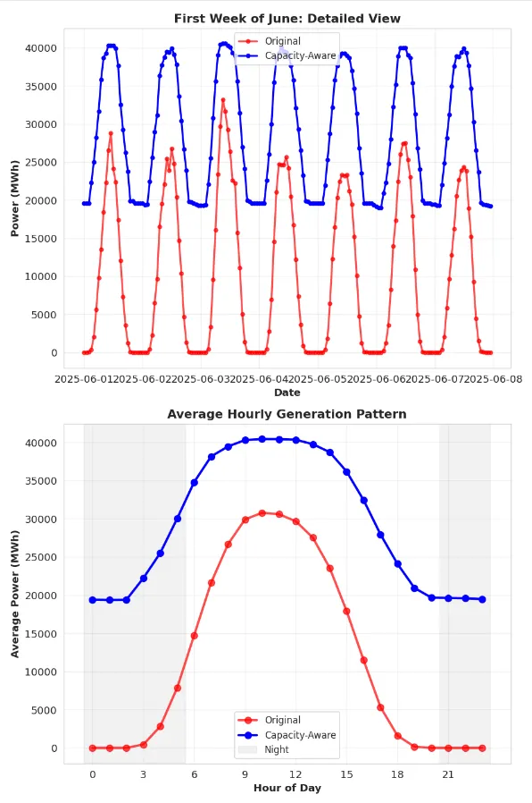
Note: I still don’t know if this is the correct approach or if these forecasts are close to the true values — I don’t have ground-truth data for June 2025. What I do know is that the original setup was clearly underestimating production by ignoring capacity growth, and this revised approach is at least an explicit attempt to correct that deficiency.