Towards a Theory of Bulk Orchestration

It’s a key feature of living systems, perhaps even in some ways the key feature: that even right down to a molecular scale, things are orchestrated. Molecules (or at least large ones) don’t just move around randomly, like in a liquid or a gel. Instead, what molecular biology has discovered is that there are endless active mechanisms that in effect orchestrate what even individual molecules in living systems do. But what is the result of all that orchestration? And could there perhaps be a general characterization of what happens in systems that exhibit such “bulk orchestration”? I’ve been wondering about these questions for some time. But finally now I think I may have the beginnings of some answers.

The central idea is to consider the effect that “being adapted for an overall purpose” has on the underlying operation of a system. At the outset, one might imagine that there’d be no general answer to this, and that it would always depend on the specifics of the system and the purpose. But what we’ll discover is that there is in fact typically a certain universality in what happens. Its ultimate origin is the Principle of Computational Equivalence and certain universal features of the phenomenon of computational irreducibility that it implies. But the point is that so long as a purpose is somehow “computationally simple” then—more or less regardless of what in detail the purpose is—a system that achieves it will show certain features in its behavior.

Whenever there’s computational irreducibility we can think of it as exerting a powerful force towards unpredictability and randomness (as it does, for example, in the Second Law of thermodynamics). So for a system to achieve an overall “computationally simple purpose” this computational irreducibility must in some sense be tamed, or at least contained. And in fact it’s an inevitable feature of computational irreducibility that within it there must be “pockets of computational reducibility” where simpler behavior occurs. And at some level the way computationally simple purposes must be achieved is by tapping into those pockets of reducibility.

When there’s computational irreducibility it means that there’s no simple narrative one can expect to give of how a system behaves, and no overall “mechanism” one can expect to identify for it. But one can think of pockets of computational reducibility as corresponding to at least small-scale “identifiable mechanisms”. And what we’ll discover is that when there’s a “simple overall purpose” being achieved these mechanisms tend to become more manifest. And this means that when a system is achieving an overall purpose there’s a trace of this even down in the detailed operation of the system. And that trace is what I’ve called “mechanoidal behavior”—behavior in which there are at least small-scale “mechanism-like phenomena” that we can think of as acting together through “bulk orchestration” to achieve a certain overall purpose.

The concept that there might be universal features associated with the interplay between some kind of overall simplicity and underlying computational irreducibility is something not unfamiliar. Indeed, in various forms it’s the ultimate key to our recent progress in the foundations of physics, mathematics and, in fact, biology.

In our effort to get a general understanding of bulk orchestration and the behavior of systems that “achieve purposes” there’s an analogy we can make to statistical mechanics. One might have imagined that to reach conclusions about, say, gases, we’d have to have detailed information about the motion of molecules. But in fact we know that if we just consider the whole ensemble of possible configurations of molecules, then by taking statistical averages we can deduce all sorts of properties of gases. (And, yes, the foundational reason this works we can now understand in terms of computational irreducibility, etc.)

So could we perhaps do something similar for bulk orchestration? Is there some ensemble we can identify in which wherever we look there will with overwhelming probability be certain properties? In the statistical mechanics of gases we imagine that the underlying laws of mechanics are fixed, but there’s a whole ensemble of possible initial configurations for the molecules—almost all of which turn out to have the same limiting features. But in biology, for example, we can think of different genomes as defining different rules for the development and operation of organisms. And so now what we want is a new kind of ensemble—that we can call a rulial ensemble: an ensemble of possible rules.

But in something like biology, it’s not all possible rules we want; rather, it’s rules that have been selected to “achieve the purpose” of making a successful organism. We don’t have a general way to characterize what defines biological fitness. But the key point here is that at a fundamental level we don’t need that. Instead it seems that just knowing that our fitness function is somehow computationally simple tells us enough to be able to deduce properties of our “rulial ensemble”.

But are the fitness functions of biology in fact computationally simple? I’ve recently argued that their simplicity is precisely what makes biological evolution possible. Like so many other foundational phenomena, it seems that biological evolution is a reflection of the interplay between computational simplicity—in the case of fitness functions—and underlying computational irreducibility. (In effect, organisms have a chance only because the problems they have to solve aren’t too computationally difficult.) But now we can use the simplicity of fitness functions—without knowing any more details about them—to make conclusions about the relevant rulial ensemble, and from there to begin to derive general principles associated with bulk orchestration.

When one describes why a system does what it does, there are two different approaches one can take. One can go from the bottom up and describe the underlying rules by which the system operates (in effect, its “mechanism”). Or one can go from the top down and describe what the system “achieves” (in effect, its “goal” or “purpose”). It tends to be difficult to mix these two approaches. But what we’re going to find here is that by thinking in terms of the rulial ensemble we will be able to see the general pattern of both the “upward” effect of underlying rules, and the “downward” effect of overall purposes.

What I’ll do here is just a beginning—a first exploration, both computational and conceptual, of the rulial ensemble and its consequences. But already there seem to be strong indications that by thinking in terms of the rulial ensemble one may be able to develop what amounts to a foundational theory of bulk orchestration, and with it a foundational theory of certain aspects of adaptive systems, and most notably biology.

Some First Examples

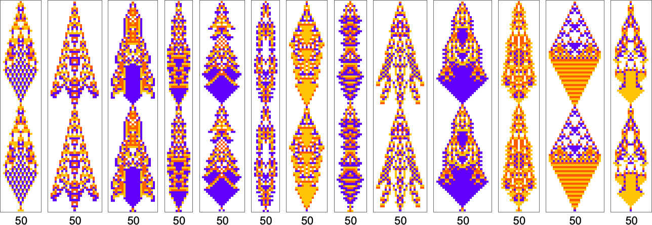
To begin our explorations and start developing our intuition let’s look at a few simple examples. We’ll use the same basic framework as in my recent work on biological evolution. The idea is to have cellular automata whose rules serve as an idealization of genotypes, and whole behavior serves as an idealization of the development of phenotypes. For our fitness function we’re going to start with something very specific: that after 50 steps (starting from a single-cell “seed”) our cellular automaton should generate “output” that consists of three equal blocks of cells colored red, blue and yellow.

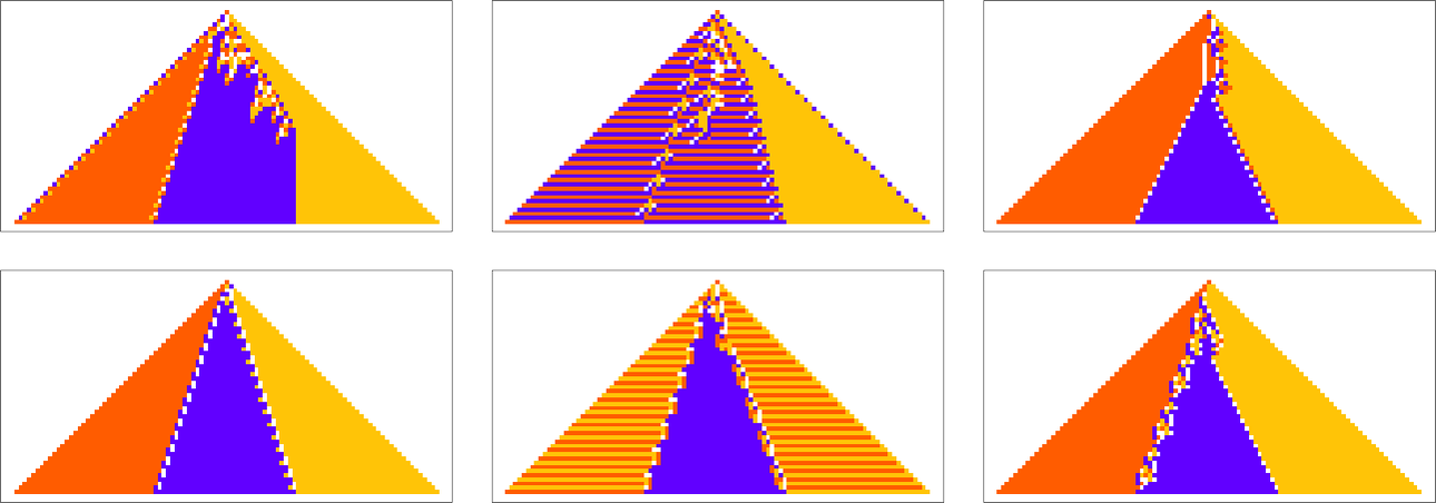
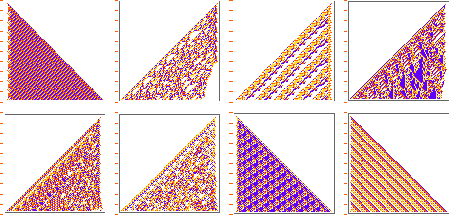
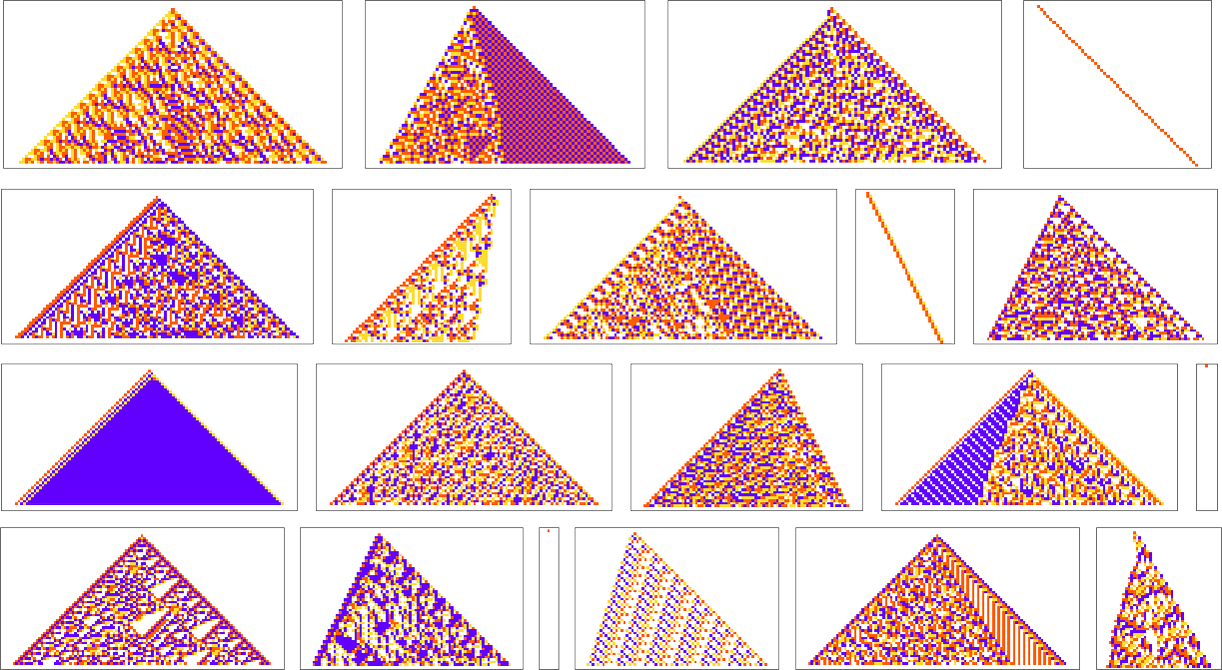
Here are some examples of rules that “solve this particular problem”, in various different ways:

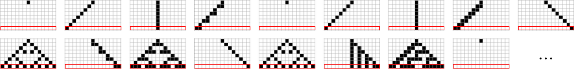
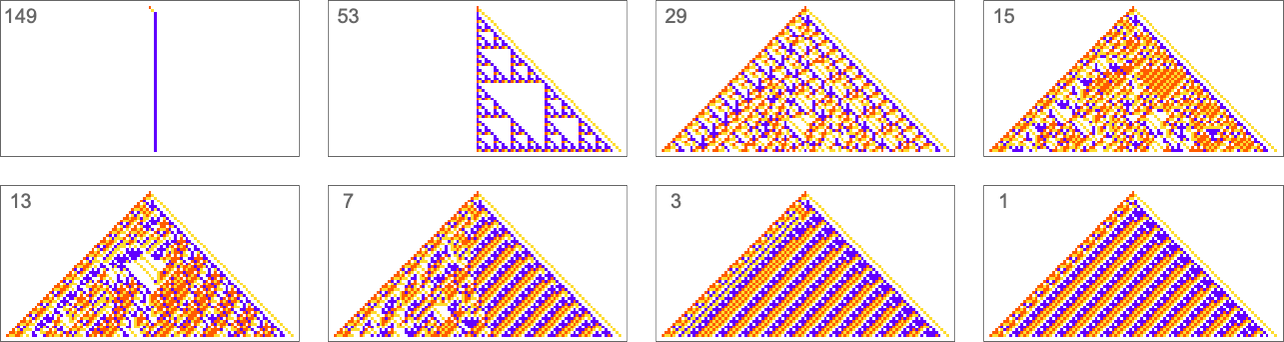
How can such rules be found? Well, we can use an idealization of biological evolution. Let’s consider the first rule above:

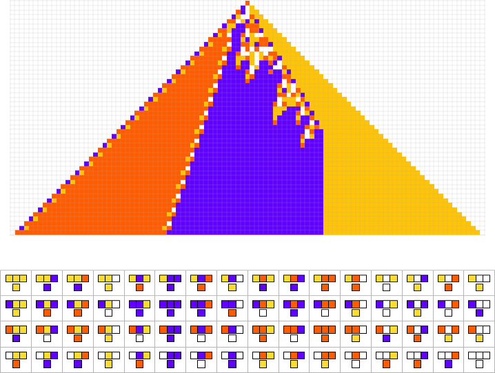
We start, say, from a null rule, then make successive random point mutations in the rule

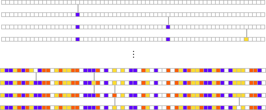
keeping those mutations that don’t take us further from achieving our goal (and dropping those that do, each indicated here by a red dot):

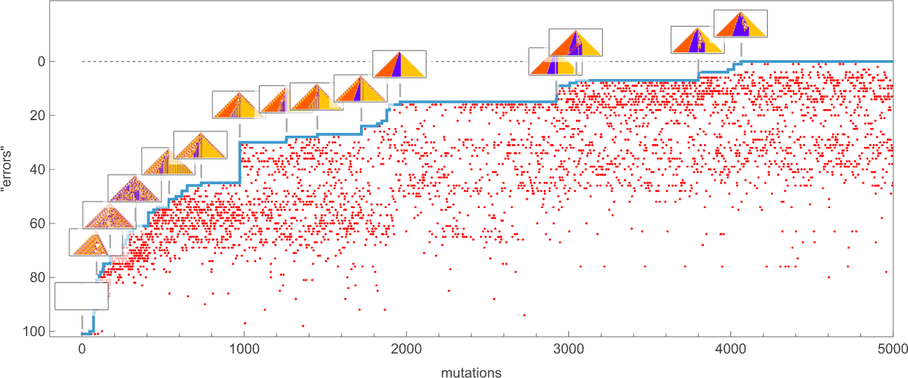
The result is that we “progressively adapt” over the course of a few thousand mutations to successively reduce the number of “errors” and eventually (and in this case, perfectly) achieve our goal:

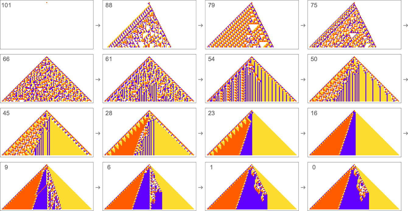
Early in this sequence there’s lots of computational irreducibility in evidence. But in the process of adapting to achieve our goal the computational irreducibility progressively gets “contained” and in effect squeezed out, until eventually the final solution in this case has an almost completely simple structure.

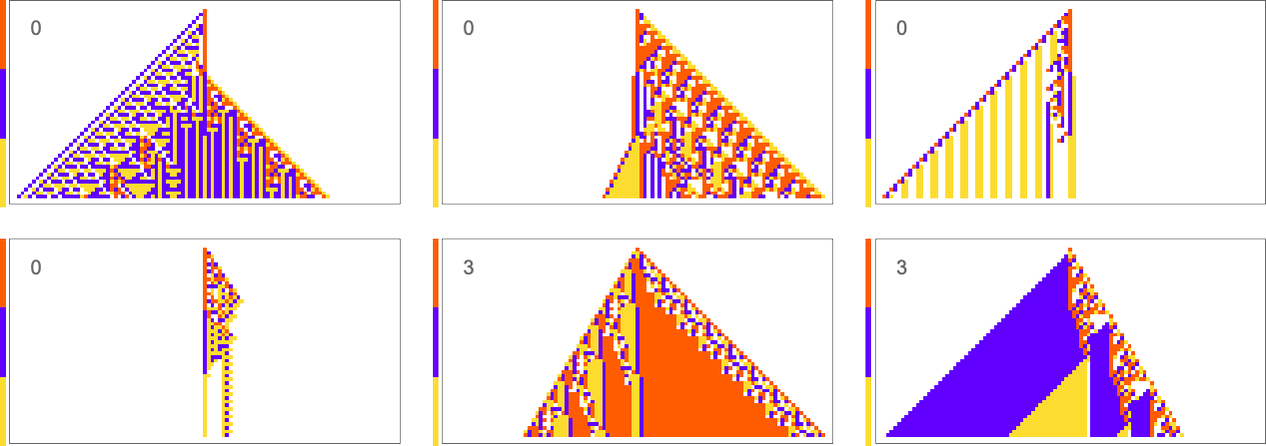
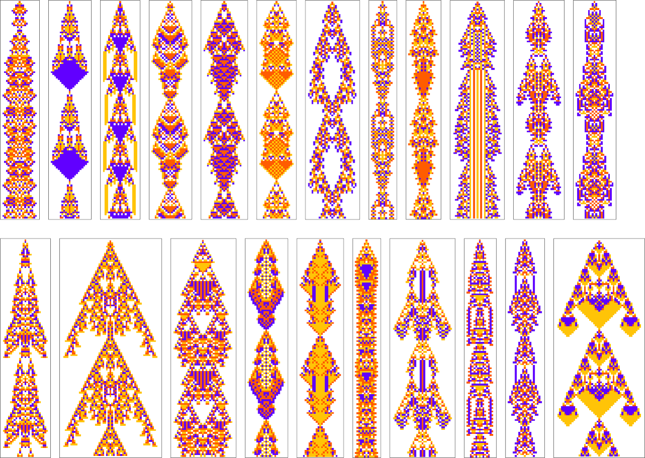
The example we’ve just seen succeeds in exactly achieving the objective we defined—though it takes about 4000 steps of adaptive evolution to do so. But if we limit the number of steps of adaptive evolution then in general we won’t be able to reach the exact objective we’ve defined. But here are some results we get with 10,000 steps of adaptive evolution (sorted by how close they get):

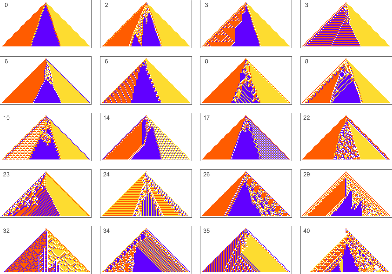
In all cases there’s a certain amount of “identifiable mechanism” to what these rules do. Yes, there can be patches of complex—and presumably computationally irreducible—behavior. But particularly the rules that do better at achieving our exact objective tend to “keep this computational irreducibility at bay”, and emphasize their “simple mechanisms”.

So what we see is that among all possible rules, those that get even close to achieving the “purpose” we have set in effect show at least “patches of mechanism”. In other words, the imposition of a purpose selects out rules that “exhibit mechanism”, and show what we’ve called mechanoidal behavior.

The Concept of Mutational Complexity

In the last section we saw that adaptive evolution can find (4-color) cellular automaton rules that generate the particular output we specified. But what about other kinds of output?

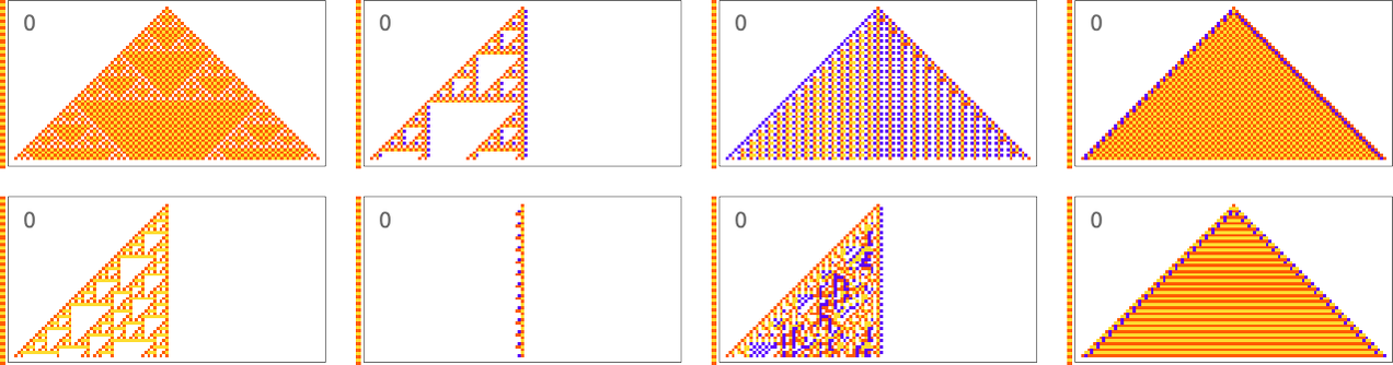
What we manage to get will depend on how much “effort” of adaptive evolution we put in. If we limit ourselves to 10,000 steps of adaptive evolution here are some examples of what happens:

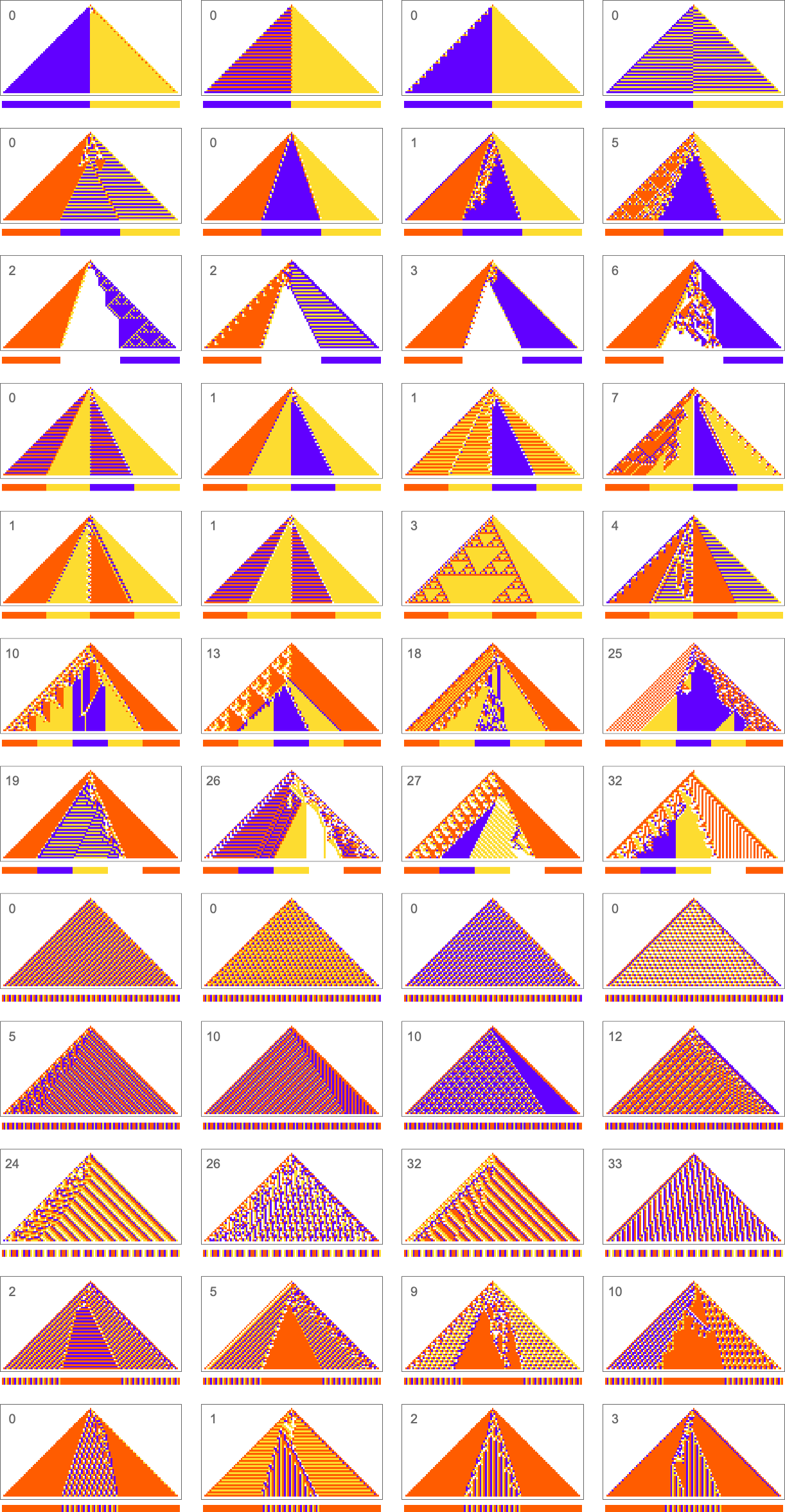
At a qualitative level the main takeaway here is that it seems that the “simpler” the objective is, the more closely it’s likely to be achieved by a given number of steps of adaptive evolution.

Looking at the first (i.e. “ultimately most successful”) examples above, here’s how they’re reached in the course of adaptive evolution:

And we see that the “simpler” sequences are reached both more successfully and more quickly; in effect they seem to be “easier” for adaptive evolution to generate.

But what do we mean by “simpler” here? In qualitative terms we can think of the “simplicity” of a sequence as being characterized by how short a description we can find of it. We might try to compress the sequence, say using some standard practical compression technique, like run-length encoding, block encoding or dictionary encoding. And for the sequences we’re using above, these will (mostly) agree about what’s simpler and what’s not. And then what we find is that sequences that are “simpler” in this kind of characterization tend to be ones that are easier for adaptive evolution to produce.

But, actually, our study of adaptive evolution itself gives us a way to characterize the simplicity—or complexity—of a sequence: we can consider a sequence more complex if the typical number of mutations it takes to come up with a rule to generate the sequence is larger. And we can define this number of mutations to be what we can call the “mutational complexity” of a sequence.

There are lots of details in tightening up this definition. But in some sense what we’re saying is that we can characterize the complexity of a sequence by how hard it is for adaptive evolution to get it generated.

To get more quantitative we have to address the issue that if we run adaptive evolution multiple times, it’ll generally take different numbers of steps to be able to get a particular sequence generated, or, say, to get to the point where there are fewer than m “errors” in the generated sequence. And, sometimes, by the way, a particular run of adaptive evolution might “get stuck” and never be able to generate a particular sequence—at least (as we’ll discuss below) with the kind of rules and single point mutations we’re using here.

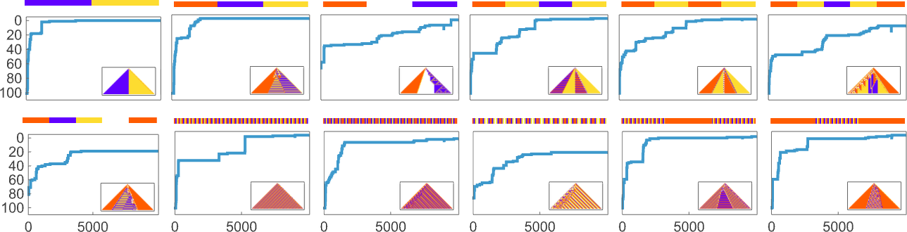
But we can still compute the probability—across many runs of adaptive evolution—to have reached a specified sequence within m errors after a certain number of steps. And this shows how that probability builds up for the sequences we saw above:

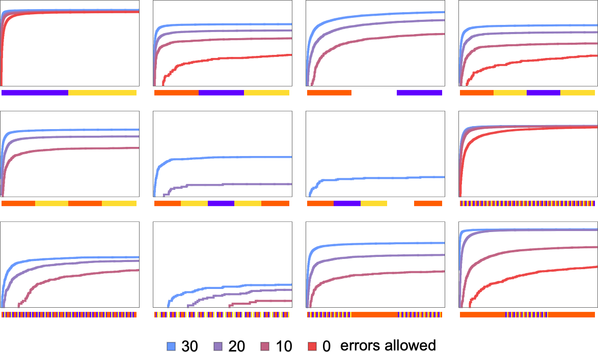
And we immediately see more quantitatively that some sequences are faster and easier to reach than others.

We can go even further by computing in each case the median number of adaptive steps needed to get “within m errors” of each sequence:

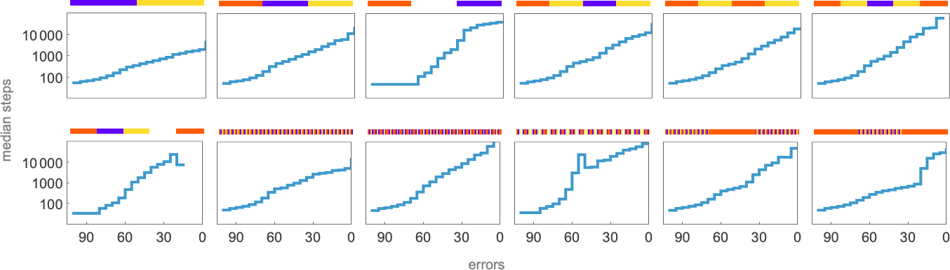
Picking a certain “desired fidelity” (say allowing a maximum of 20 errors) we then get at least one estimate of mutational complexity for our sequences:

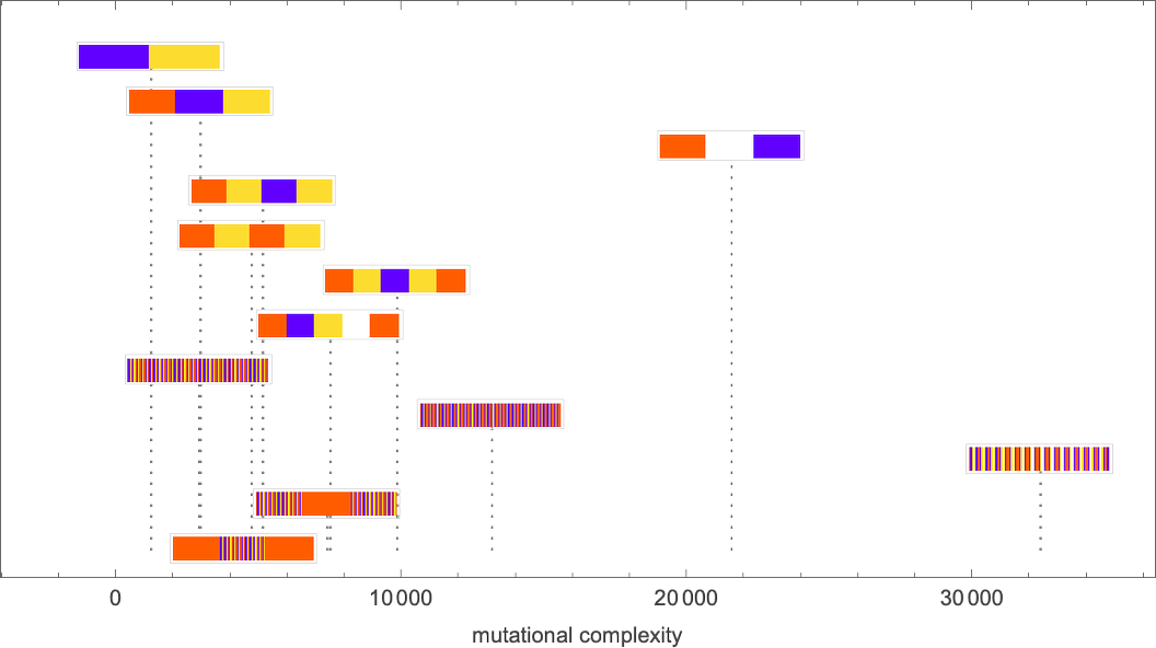
Needless to say, these kinds of numerical measures are at best a very coarse way to characterize the difficulty of being able to generate a given sequence through rules produced by adaptive evolution. And, for example, instead of just looking at the probability to reach a given “fidelity” we could be looking at all sorts of distributions and correlations. But in developing our intuition about the rulial ensemble it’s useful to see how we can derive even an admittedly coarse specific numerical measure of the “difficulty of reaching a sequence” through adaptive evolution.

Possible and Impossible Objectives

We’ve seen above that some sequences are easier to reach by adaptive evolution than others. But can any sequence we might look for actually be found at all? In other words—regardless of whether adaptive evolution can find it—is there in fact any cellular automaton rule at all (say a 4-color one) that successfully generates any given sequence?

It’s easy to see that in the end there must be sequences that can’t be generated in this way. There are 443 possible 4-color cellular automaton rules. But even though that’s a large number, the number of possible 4-color length-101 sequences is still much larger: 4101 ≈ 1061. So that means it’s inevitable that some of these sequences will not appear as the output from any 4-color cellular automaton rule (run from a single-cell initial condition for 50 steps). (We can think of such sequences as having too high an “algorithmic complexity” to be generated from a “program” as short as a 4-color cellular automaton rule.)

But what about sequences that are “simple” with respect to our qualitative criteria above? Whenever we succeeded above in finding them by adaptive evolution then we obviously know they can be generated. But in general this is a quintessential computationally irreducible question—so that in effect the only way to know for sure whether there’s any rule that can generate a particular sequence is just to explicitly search through all ≈ 1038 possible rules.

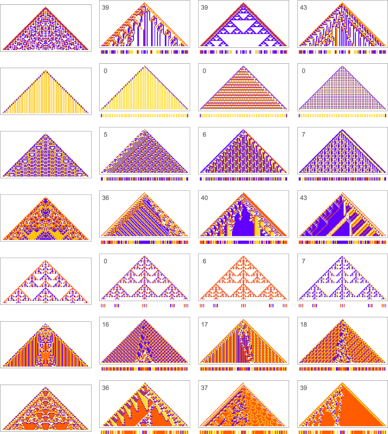
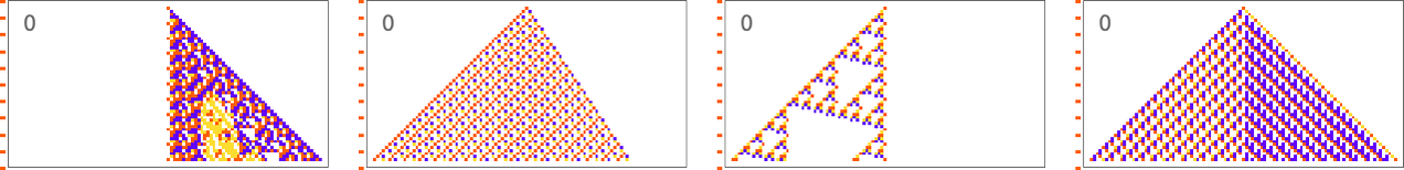
We can get some intuition, however, by looking at much simpler cases. Consider, for example, the 128 (quiescent) “elementary” cellular automata (with k = 2, r =1):

The number of distinct sequences they can generate after t steps quickly stabilizes (the maximum is 32)

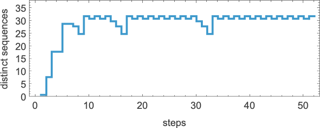
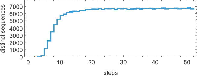
but this is soon much smaller than the total number of possible sequences of the same length (22t + 1). (The “down wiggles” are associated with additive rules like 90 and 150 generating almost blank sequences at steps of the form 2m.) Here’s the corresponding result for k = 2, r = 3/2 rules:

So what are the sequences that get “left out” by cellular automata? Already by step 2 a quiescent elementary cellular automaton can only produce 14 of the 32 possible sequences—with sequences such as and being among those excluded. One might think that one would be able to characterize excluded sequences by saying that certain fixed blocks of cells could not occur at any step in any rule. And indeed that happens for the r = 1/2 rules. But for the quiescent elementary cellular automata—with r = 1—it seems as if every block of any given size well eventually occur, presumably courtesy of the likes of rule 30.

What about, say, periodic sequences? Here are some examples that no quiescent elementary cellular automaton can generate:

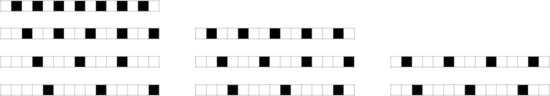
And, yes, these are, by most standards, quite “simple” sequences. But they just happen not to be “simple” for elementary cellular automata. And indeed we can expect that there will be plenty of such “coincidentally unreachable” but “seemingly simple” sequences even for our 4-color rules. But we can also expect that even if we can’t precisely reach some objective sequence, we’ll still be able to get to a sequence that is close. (The minimum “error” is, for example, 4 cells out of 15 for the first sequence above, and 2 for the last sequence).

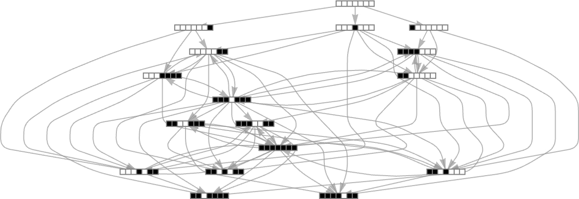
But there still remains the question of whether adaptive evolution will be able to find such sequences. For the very simple case of quiescent elementary cellular automata we can readily map out the complete multiway graph of all possible mutations between rules. Here’s what we get if we run all possible rules for 3 steps, then show possible outcomes as nodes, and possible mutations between rules as edges (the edges are undirected, because every mutation can go either way):

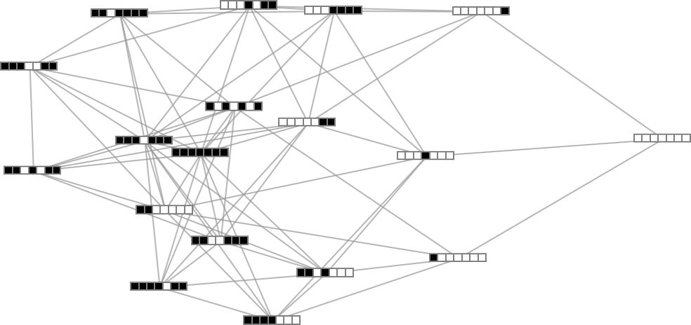
That this graph has only 18 nodes reflects the fact that quiescent elementary cellular automata can produce only 18 of the 128 possible length-7 sequences. But even within these 18 sequences there are ones that cannot be reached through the adaptive evolution process we are using.

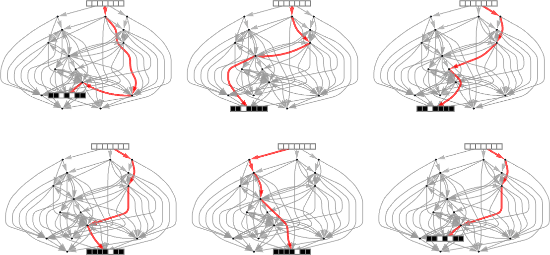
For example, let’s say our goal is to generate the sequence (or, rather, to find a rule that will do so). If we start from the null rule—which generates —then our adaptive evolution process defines a foliated version of the multiway graph above:

Starting from some paths (i.e. sequences of mutations) successfully reach . But this only happens about 25% of the time. The rest of the time the adaptive process gets stuck at or and never reaches :

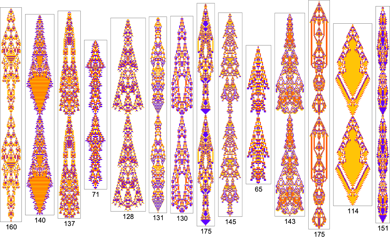
So what happens if we look at larger cellular automaton rule spaces? In such cases we can’t expect to trace the full multiway graph of possible mutations. And if we pick a sequence at random as our target, then for a long sequence the overwhelming probability is that it won’t be reachable at all by any cellular automaton with a rule of a given type. But if we start from a rule—say picked at random—and use its output as our target, then this guarantees that there’s at least one rule that produces this sequence. And then we can ask how difficult it is for adaptive evolution to find a rule that works (most likely not the original one).

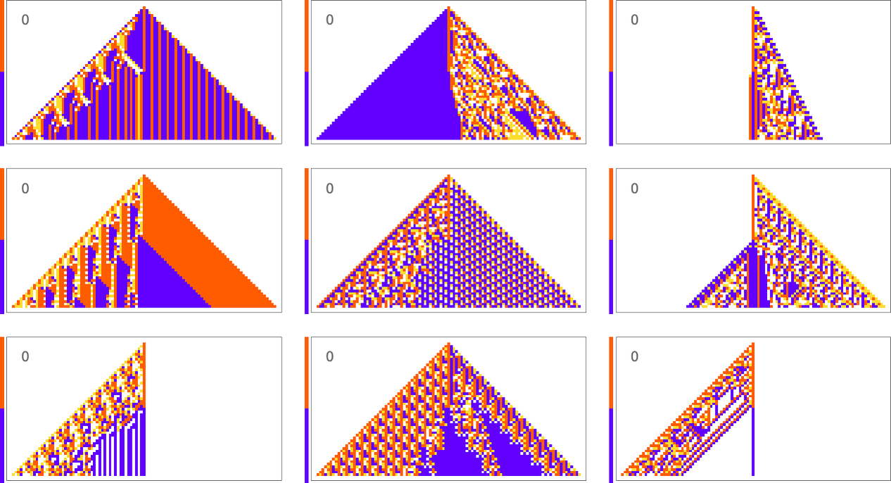
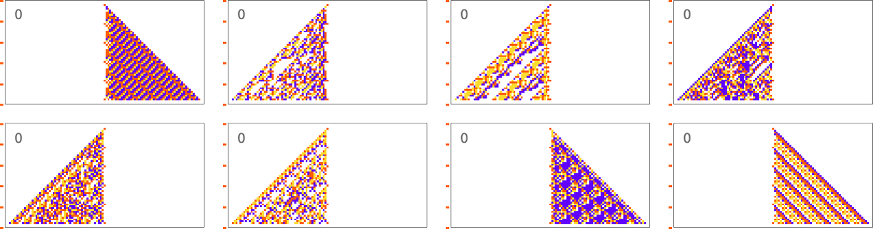
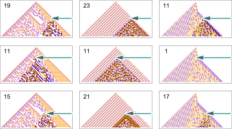
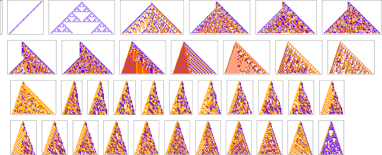
Here are some examples—with the original rule on the left, and the best results found from 10,000 steps of adaptive evolution on the right:

What we see is fairly clear: when the pattern generated by the original rule looks simple, adaptive evolution can readily find rules that successfully produce the same output, albeit sometimes in quite different ways. But when the pattern generated by the original rule is more complicated, adaptive evolution typically won’t be able to find a rule that exactly reproduces its output. And so, for examples, in the cases shown here many errors remain even in the “best results” after 10,000 steps of adaptive evolution.

Ultimately this not surprising. When we pick a cellular automaton rule at random, it’ll often show computational irreducibility. And in a sense all we’re seeing here is that adaptive evolution can’t “break” computational irreducibility. Or, put another way, computationally irreducible processes generate mutational complexity.

Other Objective Functions

In everything we’ve done so far we’ve been considering a particular type of “goal”: to have a cellular automaton produce a specified arrangement of cells after a certain number of steps. But what about other types of goals? We’ll look at several here. The general features of what will happen with them follow what we’ve already seen, but each will show some new effects and will provide some new perspectives.

Vertical Sequences

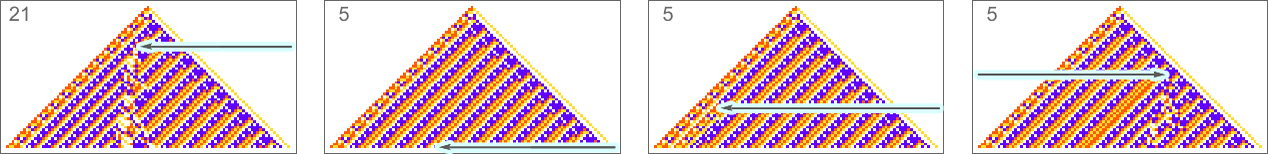
As a first example, let’s consider trying to match not the horizontal arrangement of cells, but the vertical one—in particular the sequence of colors in the center column of the cellular automaton pattern. Here’s what we get with the goal of having a block of red cells followed by an equal block of blue:

The results are quite diverse and “creative”. But it’s notable that in all cases there’s definite “mechanism” to be seen “right around the center column”. There’s all sorts of complexity away from the center column, but it’s sufficiently “contained” that the center column itself can achieve its “simple goal”.

Things are similar if we ask to get three blocks of color rather than two—though this goal turns out to be somewhat more difficult to achieve:

It’s also possible to get :

And in general the difficulty of getting a particular vertical sequence of blocks tends to track the difficulty of getting the corresponding horizontal sequence of blocks. Or, in other words, the pattern of mutational complexity seems to be similar for sequences associated with horizontal and vertical goals.

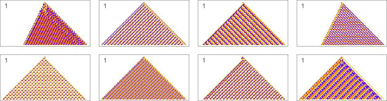
This also seems to be true for periodic sequences. Alternating colors are easy to achieve, with many “tricks” being possible in this case:

A sequence with period 5 is pretty much the same story:

When the period gets more comparable to the number of cellular automaton steps that we’re sampling it for, the “solutions” get wilder:

And some of them are quite “fragile”, and don’t “generalize” beyond the original number of steps for which they were adapted:

Color Frequencies in Output

The types of goals we’ve considered so far have all involved trying to get exact matches to specified sequences. But what if we just ask for an average result? For example, what if we ask for all 4 colors to occur with equal frequency in our output, but allow them to be arranged in any way? With the same adaptive evolution setup as before we rather quickly find “solutions” (where because we’re running for 50 steps and getting patterns of width 101, we’re always “off by at least 1” relative to the exact 25:25:25:25 result):

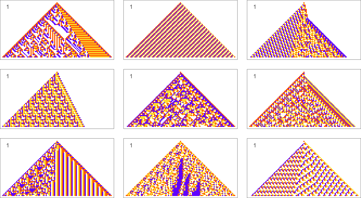
A few of these solutions seem to have “figured out a mechanism” to get all colors equally. But others seem like they just “happen to work”. And indeed, taking the first three cases here, this shows the relative numbers of cells of different colors obtained at successive steps in running the cellular automaton:

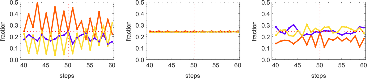
The pattern that looks simple consistently has equal numbers of each color at every step. The others just “happen to hit equality” after running for exactly 50 steps, but on either side don’t achieve equality.

And, actually, it turns out that all these solutions are in some sense quite fragile. Change the color of just one cell and one typically gets an expanding region of change—that takes the output far from color equality:

So how can we get rules that more robustly achieve our color equality objective? One approach is to force the adaptive evolution to “take account of possible perturbations” by applying a few perturbations at every adaptive evolution step, and keeping a particular mutation only if neither it, nor any of its perturbed versions, has lower fitness than before.

Here’s an example of one particular sequence of successive rules obtained in this way:

And now if we apply perturbations to the final result, it doesn’t change much:

It’s notable that this robust solution looks simple. And indeed that’s common, with a few other examples of robust, exact solutions being:

In effect it seems that requiring a robust, exact solution “forces out” computational irreducibility, leaving only readily reducible patterns. If we relax the constraint of being an exact solution even a little, though, more complex behavior quickly creeps in:

Whole-Pattern Color Frequencies

We’ve just looked at trying to achieve particular frequencies of colors in the “output” of a cellular automaton (after running for 50 steps). But what if we try to achieve certain frequencies of colors throughout the pattern produced by the cellular automaton?

For example, let’s say that our goal is to have color frequencies in the ratios: . Adaptive evolution fairly easily finds good “solutions” for this:

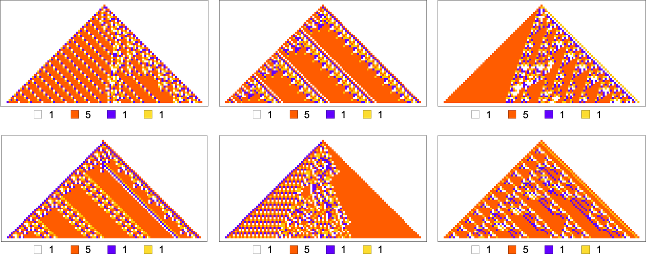
And in fact it does so for any “relative red level”:

But if we plot the median number of adaptive evolution steps needed to achieve these results (i.e. our approximation to mutational complexity) we see that there’s a systematic increase with “red level”:

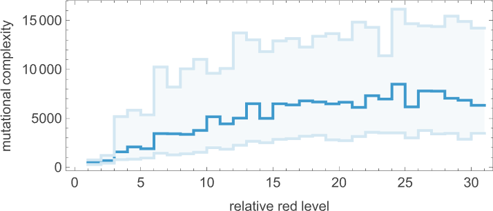
In effect, the higher the red level the “more stringent” the constraints we’re trying to satisfy are—and the more steps of adaptive evolution it takes to do that. But looking at the actual patterns obtained at different red levels, we also see something else: that as the constraints get more stringent, the pattern seems to have computational irreducibility progressively “squeezed out” of them—leaving behavior that seems more and more mechanoidal.

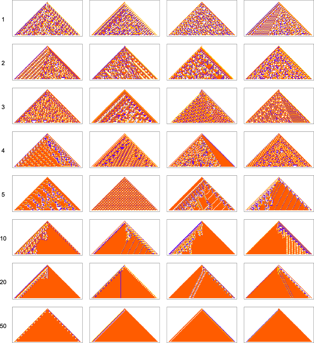
As another example along the same lines, consider goals of the form . Here are results one gets varying the “white level”:

We see two rather different approaches being taken to the “problem of having more white”. When the white level isn’t too large, the pattern just gets “airier”, with more white inside. But eventually the pattern tends to contract, “leaving room” for white outside.

Growth Shapes

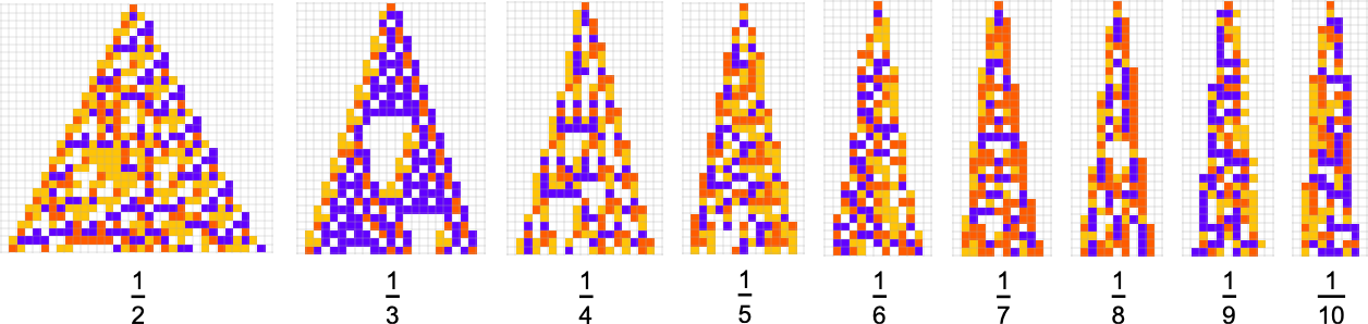
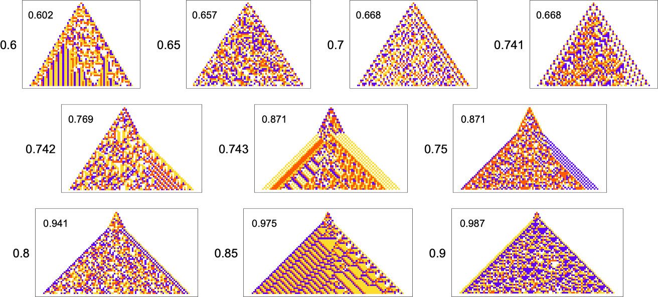
In most of what we’ve done so far, the overall “shapes” of our cellular automaton patterns have ended up always just being simple triangles that expand by one cell on each side at each step—though we just saw that with sufficiently stringent constraints on colors they’re forced to be different shapes. But what if our actual goal is to achieve a certain shape? For example, let’s say we try to get triangular patterns that grow at a particular rate on each side.

Here are some results for growth rates of the form 1/n (i.e. growing by an average of 1 cell every n steps):

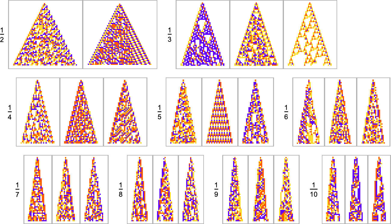
This is the sequence of adaptive evolution steps that led to the first example of growth rate

and this is the corresponding sequence for growth rate :

And although the interiors of most of the final patterns here are complicated, their outer boundaries tend to be simple—at least for small n—and in a sense “very mechanically” generate the exact target growth rate:

For larger n, things get more complicated—and adaptive evolution doesn’t typically “find an exact solution”. And if we run our “solutions” longer we see that—particularly for larger n—they often don’t “generalize” very well, and soon start deviating from their target growth rates:

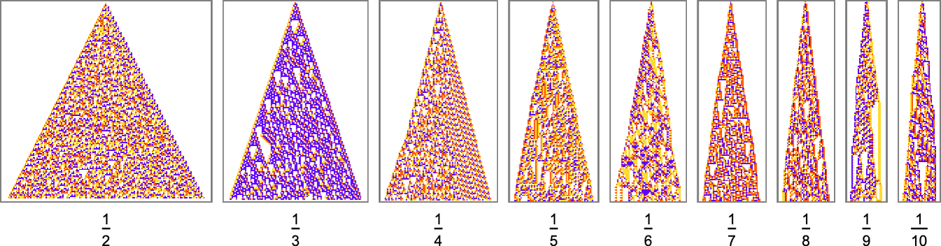
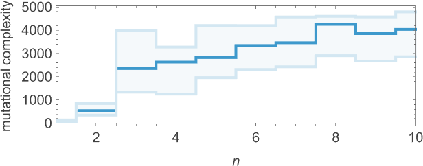
As we increase n we typically see that more steps of adaptive evolution are needed to achieve our goal, reflecting the idea that “larger n growth” has more mutational complexity:

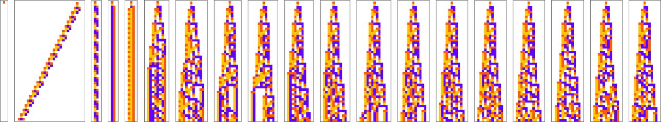
For rational growth rates like fairly simple exact solutions are possible. But for irrational growth rates, that’s no longer true. Still, it turns out that adaptive evolution is in a sense strong enough—and our cellular automaton rule space is large enough—that good approximations even to irrational growth rates can often be reached:

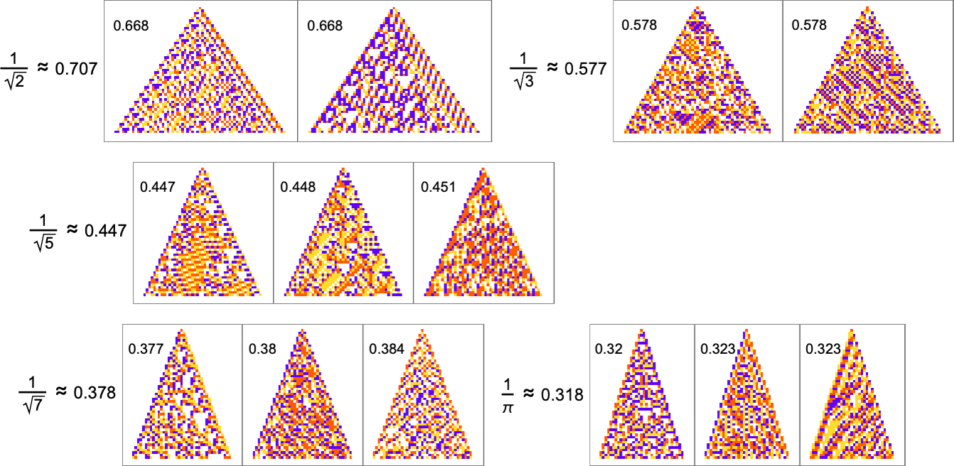
The “solutions” typically remain quite consistent when run longer:

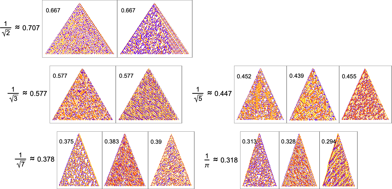
But there are still some notable limitations. For example, while a growth rate of exactly 1 is easy to achieve, growth rates close to 1 are in effect “structurally difficult”. For example, above about 0.741 adaptive evolution tends to “cheat”—adding a “hat” at the top of the pattern instead of actually producing a boundary with consistent slope:

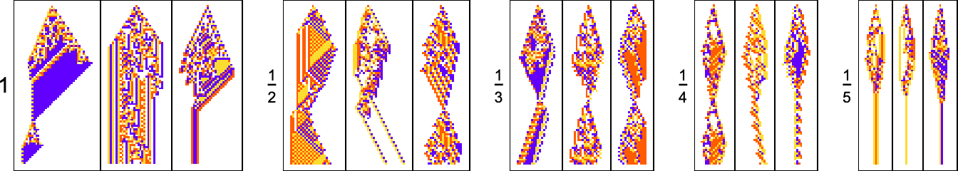
What about other shapes as goals? Here’s what happens with diamond shapes of difficult widths:

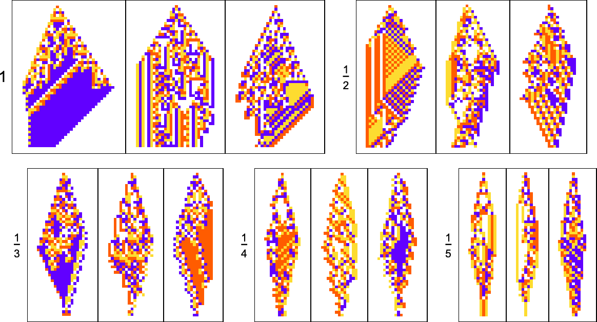
Adaptive evolution is quite constrained by what’s structurally possible in a cellular automaton of this type—and the results are not particularly good. And indeed if one attempts to “generalize” them, it’s clear none of them really “have the idea” of a diamond shape:

Lifetimes

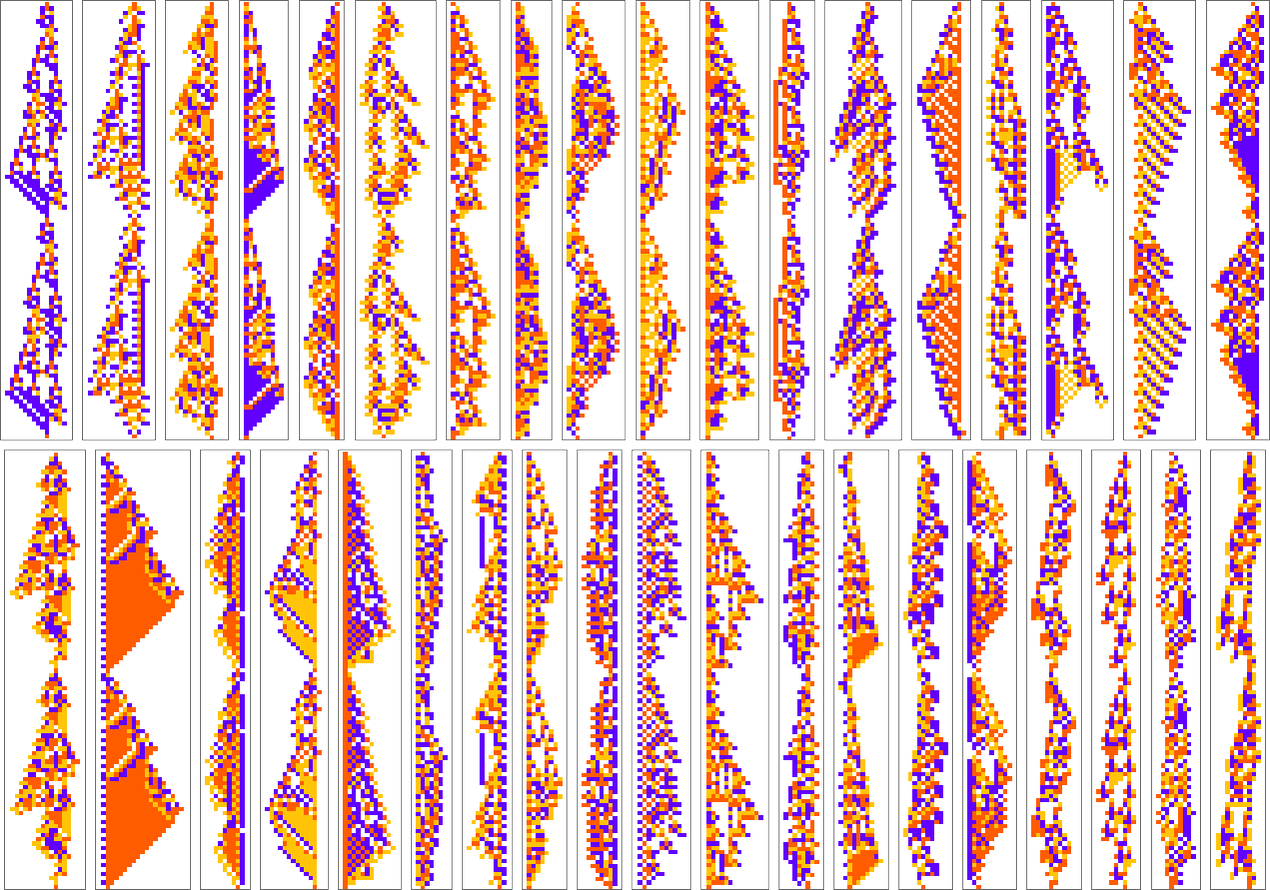
In the examples we’ve discussed so far, we’ve focused on what cellular automata do over the course of a fixed number of steps—not worrying about what they might do later. But another goal we might have—which in fact I have discussed at length elsewhere—is just to have our cellular automata produce patterns that go for a certain number of steps and then die out. So, for example, we can use adaptive evolution to find cellular automata whose patterns live for exactly 50 steps, and then die out:

Just like in our other examples, adaptive evolution finds all sorts of diverse and “interesting” solutions to the problem of living for exactly 50 steps. Some (like the last one and the yellow one) have a certain level of “obvious mechanism” to them. But most of them seem to “just work” for no “obvious reason”. Presumably the constraint of living for 50 steps in some sense just isn’t stringent enough to “squeeze out” computational irreducibility—so there is still plenty of computational irreducibility in these results.

What about mutational complexity? Approximating this, as before, by the median of the number of adaptive evolution steps—and sampling a few hundred cases for each lifetime goal (and plotting the quartiles as well as the median)—we see a systematic increase of mutational complexity as we increase the lifetime goal:

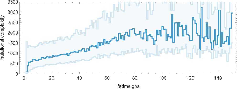
In effect this shows us that if we increase the lifetime goal, it becomes more and more difficult for adaptive evolution to reach that goal. (And, as we’ve discussed elsewhere, if we go far enough, we’ll ultimately reach the edge of what’s even in principle possible with, say, the particular type of 4-color cellular automata we’re using here.)

All the objectives we’ve discussed so far have the feature that they are in a sense explicit and fixed: we define what we want (e.g. a cellular automaton pattern that lives for exactly 50 steps) and then we use adaptive evolution to try to get it. But looking at something like lifetime suggests another possibility. Instead of our objective being fixed, our objective can instead be open ended. And so, for example, we might ask not for a specific lifetime, but to get the largest lifetime we can.

I’ve discussed this case at some length elsewhere. But how does it relate to the concept of the rulial ensemble that we’re studying here? When we have rules that are found by adaptive evolution with fixed constraints we end up with something that can be thought of as roughly analogous to things like the canonical (“specified temperature”) ensemble of traditional statistical mechanics. But if instead we look at the “winners” of open-ended adaptive evolution then what we have is more like a collection of extreme value than something we can view as typical of the “bulk of an ensemble”.

Periodicities

We’ve just looked at the goal of having patterns that survive for a certain number of steps. Another goal we can consider is having patterns that periodically repeat after a certain number of steps. (We can think of this as an extremely idealized analog of having multiple generations of a biological organism.)

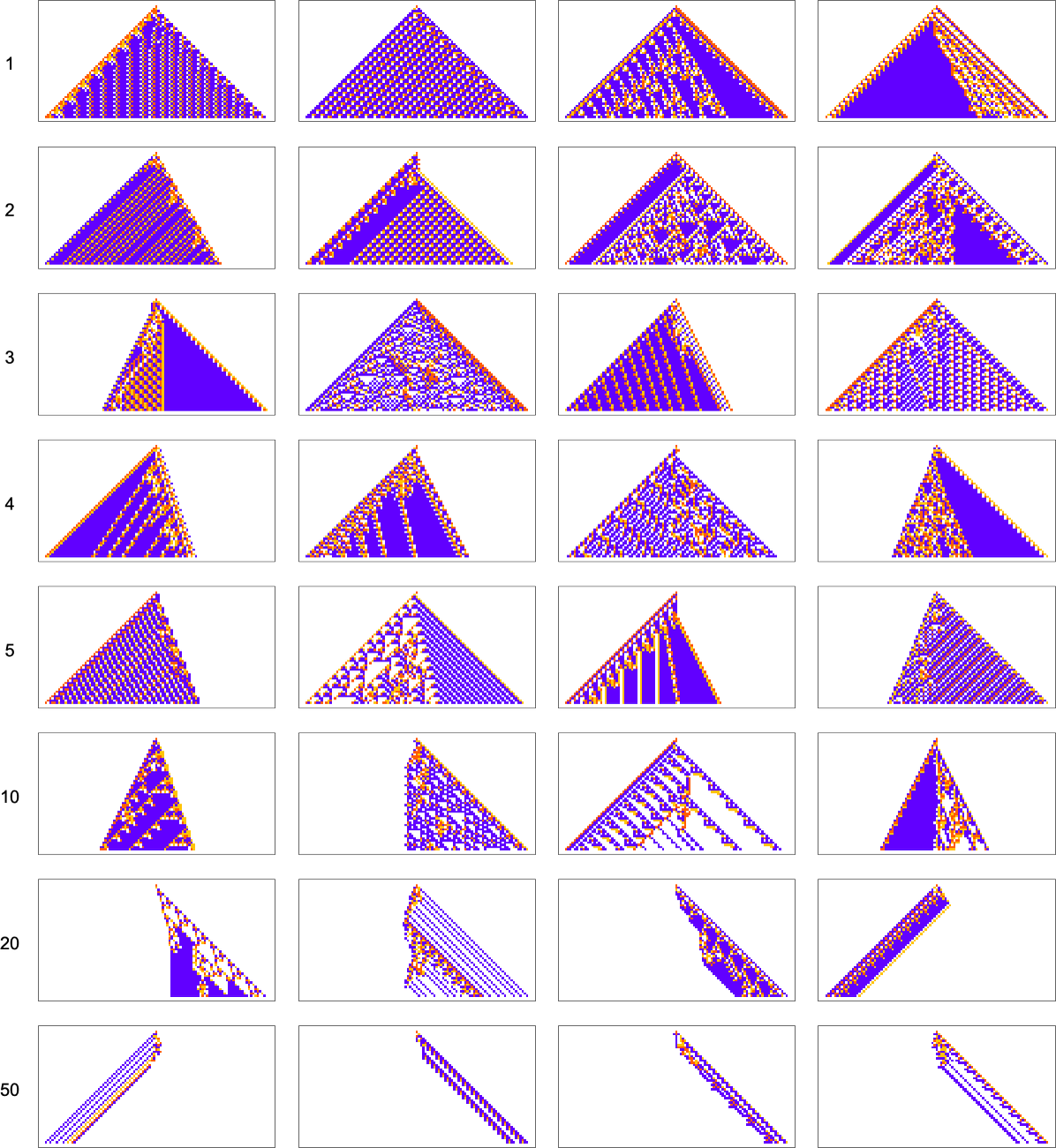
Here are examples of rules found by adaptive evolution that lead to patterns which repeat after exactly 50 steps:

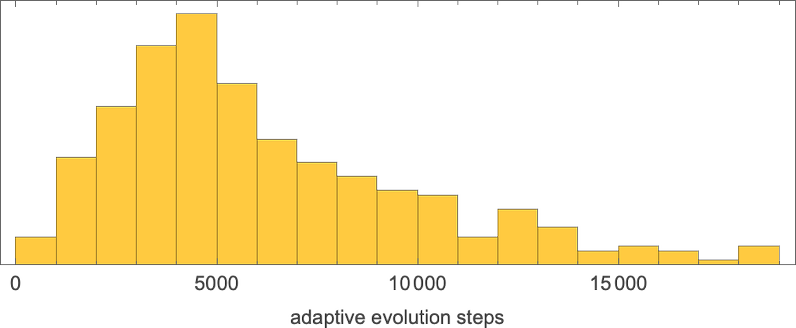
As usual, there’s a distribution in the number of steps of adaptive evolution required to achieve these results:

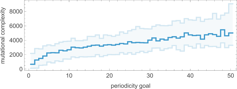
Looking at the median of the analogous distributions for different possible periods, we can get an estimate of the mutational complexity of different periods—which seems to increase somewhat uniformly with period:

By the way, it’s also possible to restrict our adaptive evolution so that it samples only symmetric rules; here are a few examples of period-50 results found in this way:

In our discussion of periodicity so far, we’ve insisted on “periodicity from the start”—meaning that after each period the pattern we get has to return to the single-cell state we started from. But we can also consider periodicity that “develops after a transient”. Sometimes the transient is short; sometimes it’s much longer. Sometimes the periodic pattern starts from a small “seed”; sometimes its seed is quite large. Here are some examples of patterns found by adaptive evolution that have ultimate period 50:

By the way, in all these cases the periodic pattern seems like the “main event” of the cellular automaton evolution. But there are other cases where it seems more like a “residue” from other behavior—and indeed that “other behavior” can in principle go on for arbitrarily long before finally giving way to periodicity:

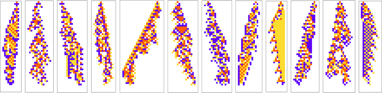
We’ve been talking so far about the objective of finding cellular automaton rules that yield patterns with specific periodicity. But just like for lifetime, we can also consider the “open-ended objective” of finding rules with the longest periods we can. And here are the best results found with a few runs of 10,000 steps of adaptive evolution (here we’re looking for periodicity without transients):

Measuring Mechanoidal Behavior

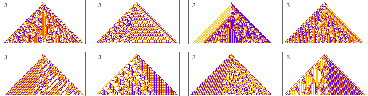
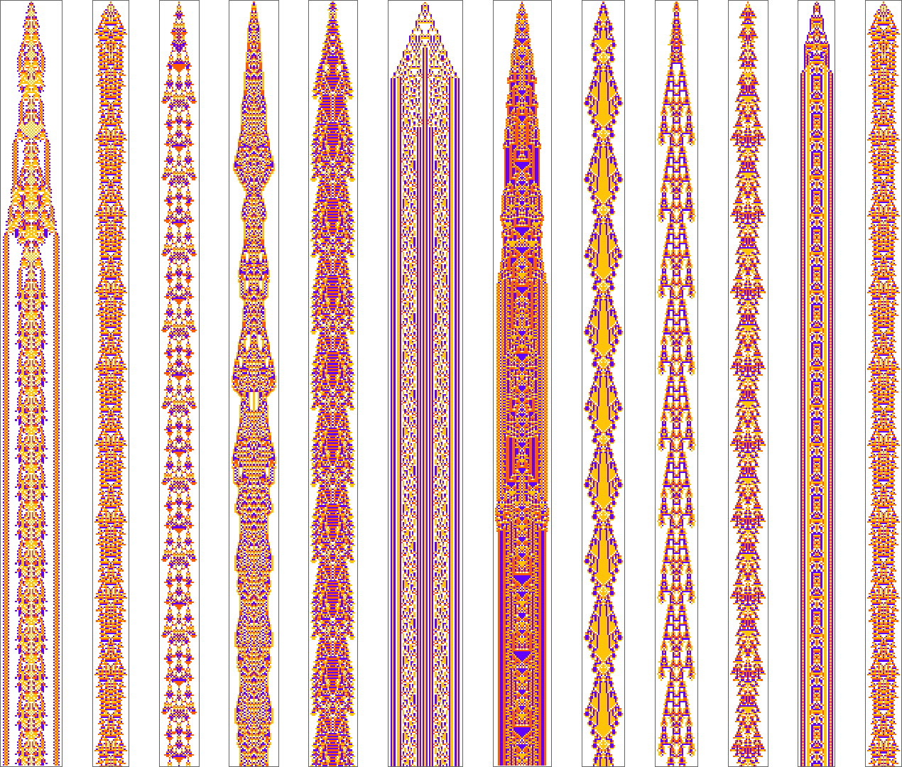
We’ve now seen lots of examples of cellular automata found by adaptive evolution. And a key question is: “what’s special about them?” If we look at cellular automata with rules chosen purely at random, here are typical examples of what we get:

Some of these patterns are simple. But many are complicated and in fact look quite random—though often with regions or patches of regularity. But what’s striking is how visually different they look from what we’ve mostly seen above in cellular automata that were adaptively evolved “for a purpose”.

So how can we characterize—and ultimately measure—that difference? Our randomly picked cellular automata seem to show either almost total computational reducibility or “unchecked computational irreducibility” (albeit usually with regions or patches of computational reducibility). But cellular automata that were successfully “evolved for a purpose” tend to look different. They tend to show what we’re calling mechanoidal behavior: behavior in which there are identifiable “mechanism-like features”, albeit usually mixed in with at least some—typically highly contained—“sparks of computational irreducibility”.

At a visual level there are typically some clear characteristics to mechanoidal behavior. For example, there are usually repeated motifs that appear throughout a system. And there’s also usually a certain degree of modularity, with different parts of the system operating at least somewhat independently. And, yes, there’s no doubt a rich phenomenology of mechanoidal behavior to be studied (closely related to the study of class 4 behavior). But at a coarse and potentially more immediately quantitative level a key feature of mechanoidal behavior is that it involves a certain amount of regularity, and computational reducibility.

So how can one measure that? Whenever there’s regularity in a system it means there’s a way to summarize what the system does more succinctly than by just specifying every state of every element of the system. Or, in other words, there’s a way to compress our description of the system.

Perhaps, one might think, one could use modularity to do this compression, say by keeping only the modular parts of a system, and eliding away the “filler” in between—much like run-length encoding. But—like run-length encoding—the most obvious version of this runs into trouble when the “filler” consists, say, of alternating colors of cells. One can also think of using block-based encoding, or dictionary encoding, say leveraging repeated motifs that appear. But it’s an inevitable feature of computational irreducibility that in the end there can never be one universally best method of compression.

But as an example, let’s just use the Wolfram Language Compress function. (Using GZIP, BZIP2, etc. gives essentially identical results.) Feed in a cellular automaton pattern, and Compress will give us a (losslessly) compressed version of it. We can then use the length of this as a measure of what’s left over after we “compress out” the regularities in the pattern. Here’s a plot of the “compressed description length” (in “Compress output bytes”) for some of the patterns we’ve seen above:

And what’s immediately striking is that the patterns “evolved for a purpose” tend to be in between patterns that come from randomly chosen rules.

(And, yes, the question of what’s compressed by what is a complicated, somewhat circular story. Compression is ultimately about making a model for things one wants to compress. And, for example, the appropriate model will change depending on what those things are. But for our purposes here, we’ll just use Compress—which is set up to do well at compressing “typical human-relevant content”.)

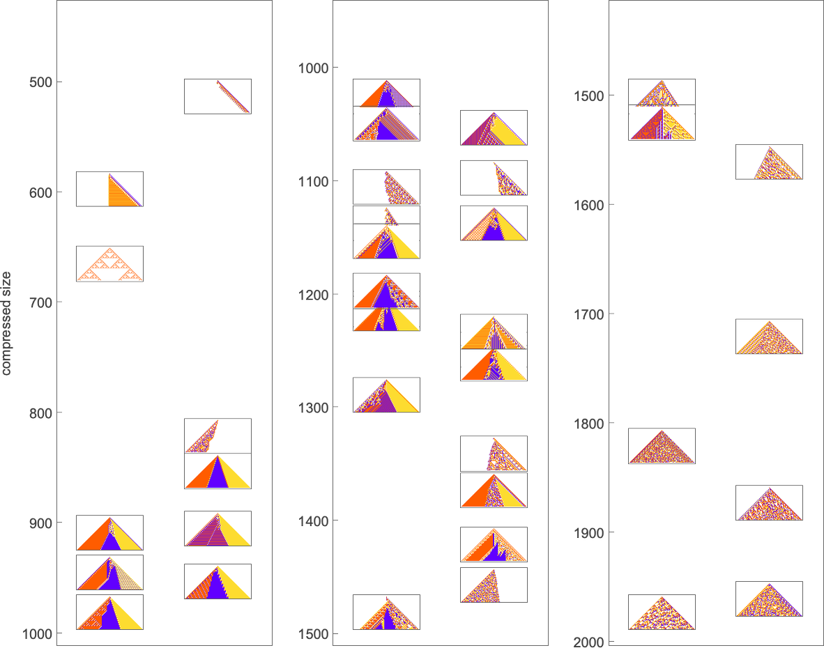
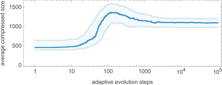
OK, so how does adaptive evolution relate to our “compressed size” measure? Here’s an example of the typical progression of an adaptive evolution process—in this case based on the goal of generating the sequence:

Given our way of starting with the null rule, everything is simple at the beginning—yielding a small compressed size. But soon the system starts developing computational irreducibility, and the compressed size goes up. Still, as the adaptive evolution proceeds, the computational irreducibility is progressively “squeezed out”—and the compressed size settles down to a smaller value.

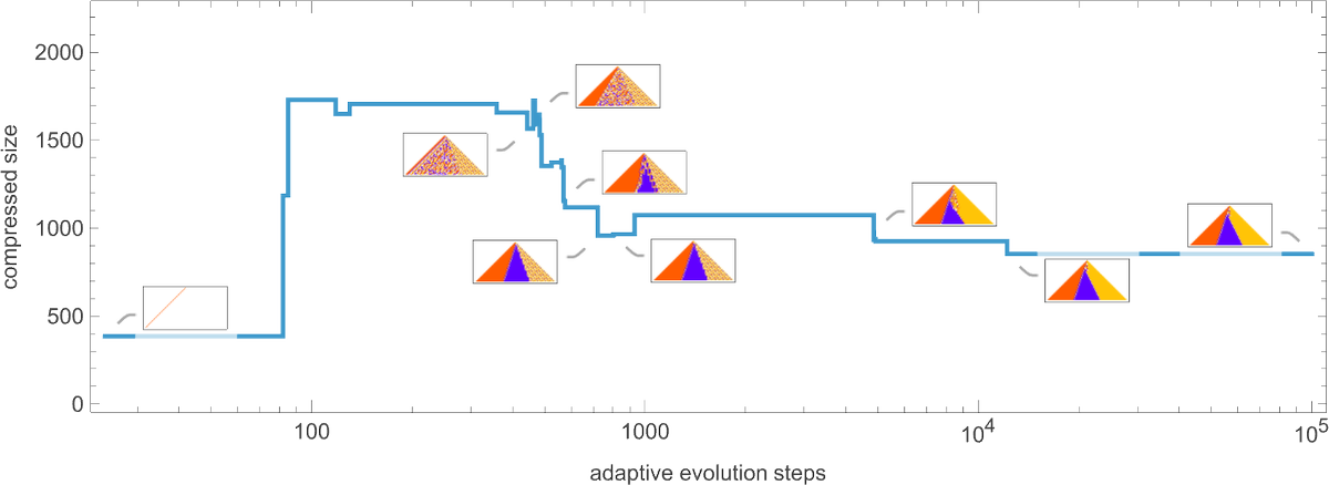
The plot above is based on a particular (randomly chosen) sequence of mutations in the underlying rule. But if we look at the average from a large collection of mutation sequences we see very much the same thing:

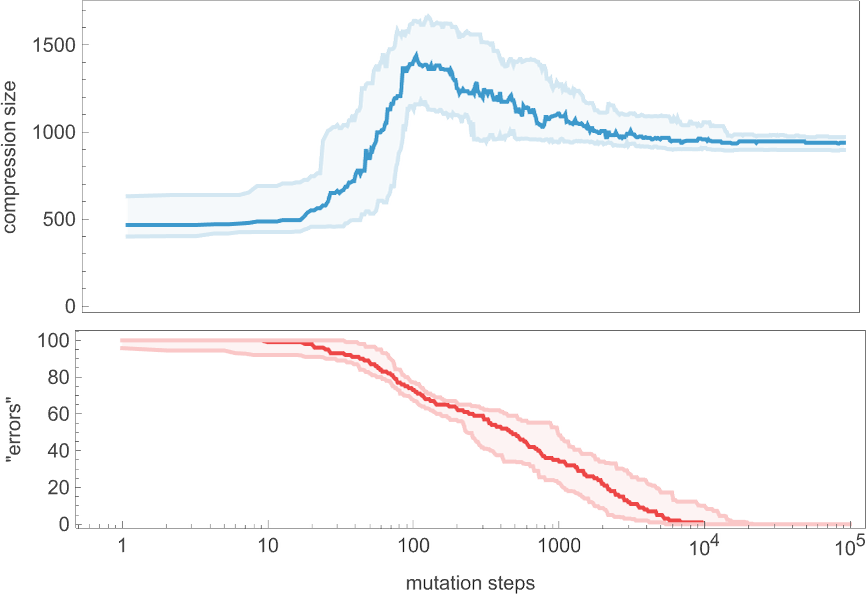
Even though the “error rate” on average goes down monotonically, the compressed size of our candidate patterns has a definite peak before settling to its final value. In effect, it seems that the system needs to “explore the computational universe” a bit before figuring out how to achieve its goal.

But how general is this? If we don’t insist on reaching zero error we get a curve of the same general shape, but slightly smoothed out (here for 20 or fewer errors):

What about for other target sequences? Here are results for all the target sequences we considered before (with the number of errors allowed in each case indicated):

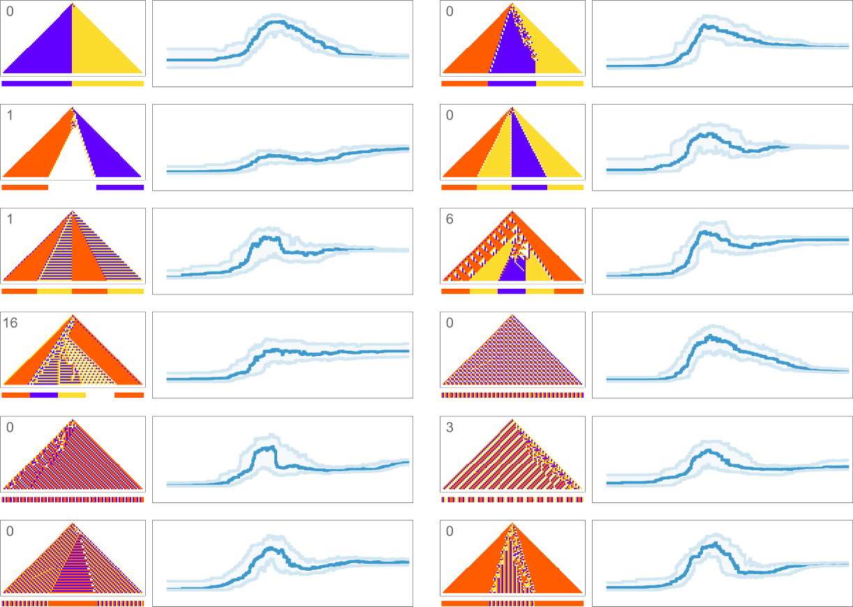
In all cases we get final compressed sizes that are much smaller than those for all-but-very-simple randomly chosen rules—indicating that our adaptive evolution process has indeed generated regularity, and our compression method has successfully picked this up.

Looking at the overall shape of the curves we’ve generated here, there seems to be a general phenomenon in evidence: the process of adaptive evolution seems to pass through a “computationally irreducible period” before getting to its final mechanoidal state. Even as it gets progressively closer to its goal, the adaptive evolution process ends up still “playing the field” before homing in on its “final solution”. (An