I’ve been spending a lot of time training neural nets lately and fortunately or unfortunately, depending on which camp you fall on, Python makes it very easy to train models.

Want to train a model? Just run model.train().

Want to calculate your loss? Just run loss = criterion(pred, target)

Want to run gradient descent? Just run loss.backward()

Call optimizer.step() and boom - your model learns.

And yet… every time I write code like this, I can’t help but feel like a sense of dissatisfaction. As if I don’t actually appreciate how easy Pytorch makes this insanely complicated process. I know there’s an enormous amount of machinery happening under the hood from computational graphs, chained gradients, parameter updates and more, and yet it’s all wrapped up in nice little function calls.

So let’s peel back the abstraction and implement it from scratch in order to really gain an appreciation of the complexity that Pytorch saves us from.

This blog walks through building a very basic autograd system in Rust called nanograd. The goal isn’t performance or completeness, it’s mainly intuition. I wanted a clearer mental model of how training loops flow forward and backward to calculate loss and gradients and update weights.

If you’ve ever wondered what really happens beneath loss.backward(), this is a great place to start.

Let’s dive in.

(Github Repo for full code)

What is Autograd?

If you’re not familiar with autograd then let’s take a minute to walk through it. If you are familiar with it and how it works in Pytorch, then you can probably skip this section.

In the Pytorch world, autograd is Pytorch’s automatic differentiation engine. What does that mean?

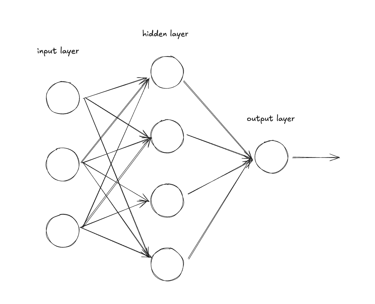
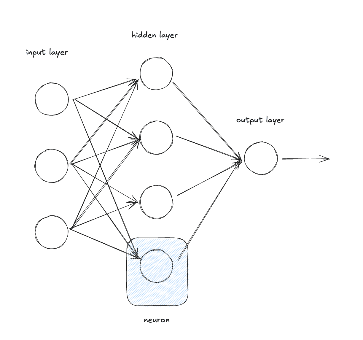
When we train neural nets, there are two main steps:

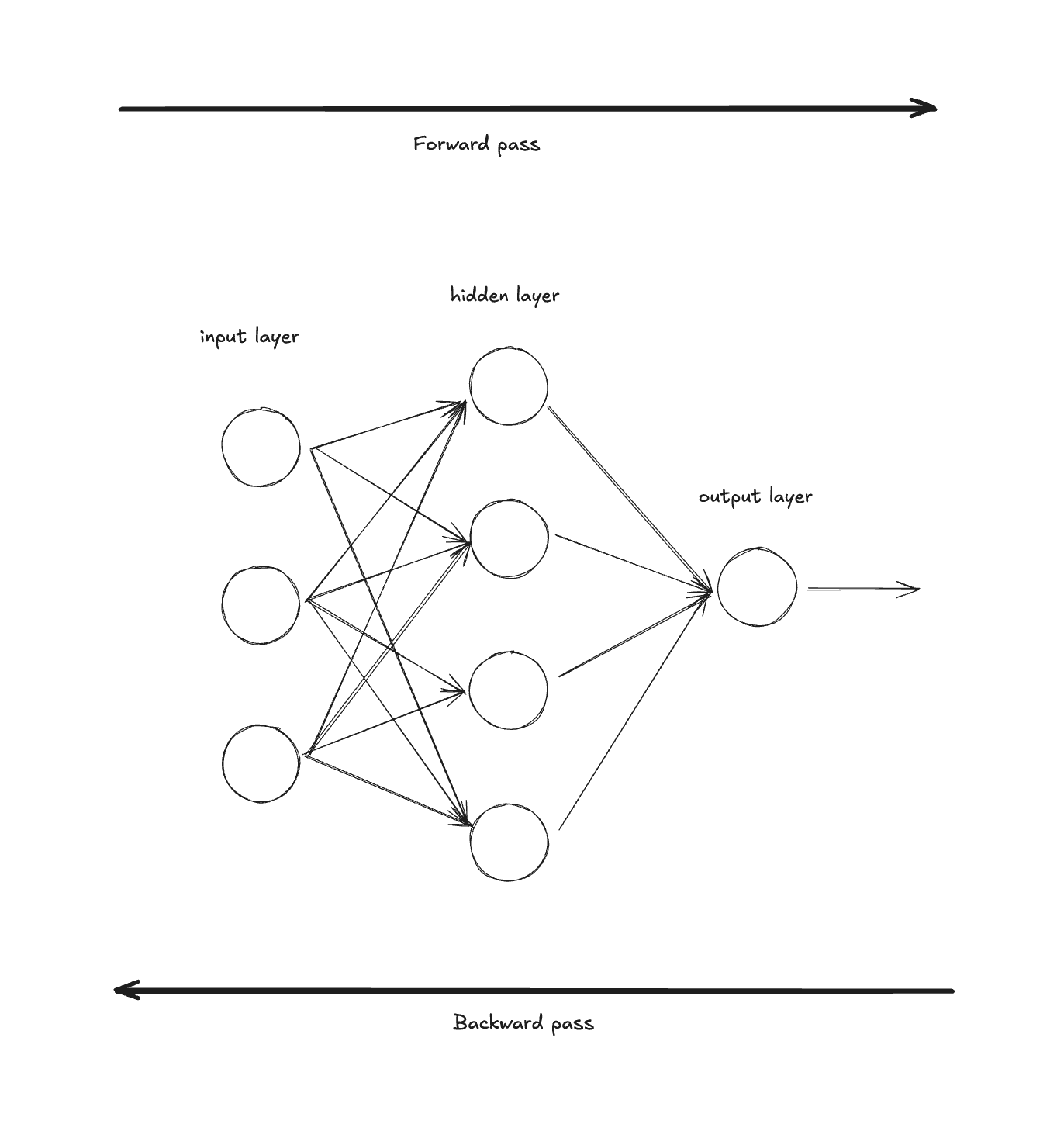
Forward pass (propagation): The neural net is fed input data and it makes predictions using its current weights. In the image above, the forward pass moves “through” the model from left (input) to right (output). At the end, we compute a loss that measures how wrong our predictions were. 1.

Backward pass (propagation): The neural net adjusts its parameters based on the loss. It does this by traversing backwards through the network (opposite of the forward pass) and calculating the gradient of the loss with respect to each parameter using the chain rule. These gradients tell us how to update each parameter to reduce the loss.

The “automatic” part means Pytorch computes these gradients for you automatically. You don’t need to manually derive and code up the derivatives for each operation in your network.

The “differentiation” part refers to computing derivatives (gradients). Specifically, autograd calculates ∂Loss/∂(every parameter) - the gradient of the loss with respect to each of the millions (or billions) of parameters in your model.

Without autograd, you’d need to manually compute and code the derivative for every operation in your network using calculus. With autograd, you just call loss.backward() and Pytorch figures it all out using the chain rule.

Autograd Main Components

We can break down an autograd system into 3 main components.

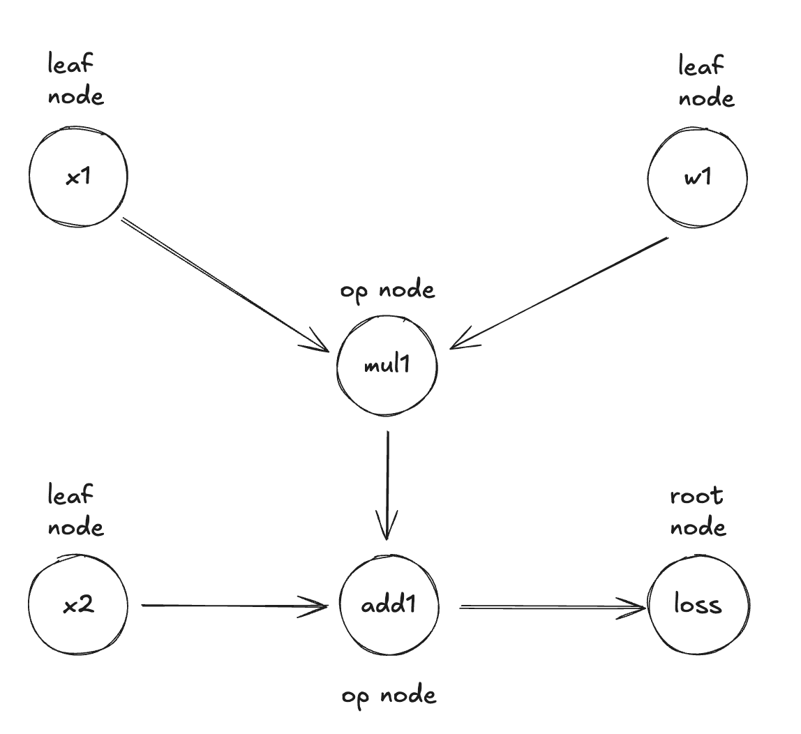
1. Computational Graph

1. Computational graph: the computational graph is a directed acyclic graph (DAG) that stores the operations of the autograd process.

• Nodes: Represent tensors (both inputs and intermediate results)
• Edges: Represent operations that transform one tensor into another
• Leaves: Input tensors and parameters (where gradients will accumulate)
• Root: The final loss value

During the forward pass, autograd does two things simultaneously:

• Runs the requested operation to compute the resulting tensor
• Records the operation’s gradient function in the DAG

During the backward pass:

• Computes the gradients from each operation’s gradient function (.grad_fn)
• Accumulates them in each tensor’s .grad attribute
• Uses the chain rule to propagate gradients all the way back to the leaf tensors

By tracing this graph from root to leaves, you can automatically compute the gradients using the chain rule.

2. Tensor Wrapper

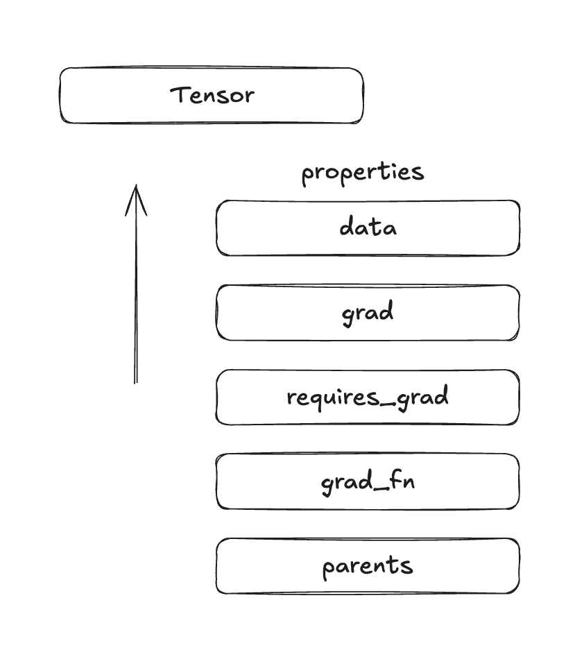
The tensor wrapper is the core data structure that makes automatic differentiation possible. It wraps the raw tensor value with metadata needed for gradient computation.

• Store the data: The actual tensor
• Track gradient requirements: A flag (requires_grad) indicating whether this tensor needs gradients computed for it
• Store accumulated gradients: A .grad field that accumulates gradients during the backward pass
• Link to computation history: A reference to the operation (grad_fn) that created this tensor
• Maintain connections: References to parent tensors

The tensor wrapper is what allows Pytorch to say “this tensor came from multiplying x by 2, so I know how to compute gradients for it.”

3. Gradient Functions

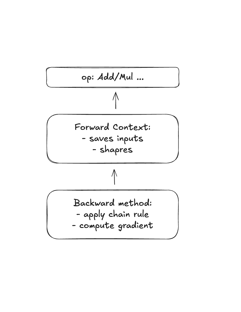
Gradient functions define how to compute derivatives for each operation. Every operation in your neural network (add, multiply, matrix multiply, ReLU, etc.) needs a corresponding gradient function.

• Store operation-specific context: Information needed to compute gradients (e.g., the input values, shapes, etc.)
• Implement the derivative: The mathematical formula for how this operation’s output gradient relates to its input gradients
• Apply the chain rule: Take the gradient flowing backwards and compute gradients for each input

Each gradient function typically needs:

1. Forward context: Data saved during the forward pass (needed for backward computation)
2. Backward method: Given the gradient of the loss with respect to the output, compute the gradient with respect to each input

Let’s look at the multiplication gradient function as an example:

Forward: z=x⋅y (save x and y for later)\textbf{Forward: } z = x \cdot y \text{ (save } x \text{ and } y \text{ for later)} Backward:\textbf{Backward:} ∂Loss∂x=∂Loss∂z×∂z∂x=∂Loss∂z×y\frac{\partial \text{Loss}}{\partial x} = \frac{\partial \text{Loss}}{\partial z} \times \frac{\partial z}{\partial x} = \frac{\partial \text{Loss}}{\partial z} \times y ∂Loss∂y=∂Loss∂z×∂z∂y=∂Loss∂z×x\frac{\partial \text{Loss}}{\partial y} = \frac{\partial \text{Loss}}{\partial z} \times \frac{\partial z}{\partial y} = \frac{\partial \text{Loss}}{\partial z} \times x

Notice how multiplication needs to save the input values (x and y) during the forward pass to compute gradients during the backward pass. This is why gradient functions need to store context.

Each operation in the computational graph has one of these gradient functions attached which forms the blueprint for the backward pass.

Autograd in Rust

Now that we have a good foundation of how autograd works and it’s main components, let’s starting spec’ing out what we’re going to build in Rust.

Here is my plan:

1. Create the core type that will wrap the number and track it’s computational history. This maps to the first and second components of the autograd system.
2. Implement a basic forward pass with addition, multiplication and power operations.
3. Implement the backward pass to compute gradients.
4. Adding non-linearities
5. Build an actual neural network using our nanograd building blocks
6. Training loop to put it all together and make sure it works.

I think this seems like a reasonable start. I’m also going to use Pytorch as a reference implementation to check out work along the way and make sure we’re getting the same output so we know we’re on the right track.

Project Scaffolding

First things first, let’s set up our project. I’m going to create a Rust project using cargo:

cargo init nanograd && cd nanograd

And then in another folder, the Pytorch equivalent to check our work:

uv init nanograd-py && cd nanograd-py source .venv/bin/activate uv add torch

I could just group them into the same project with different sub directories, but I don’t want to commit the python project. It’s really just meant as a tool, the code has no functional use.

Okay, cool, we have our projects set up.

Let’s get started with the first step: creating the core type that will wrap our tensors number and track it’s computational history.

Creating the Core Type

What does this need to store? Here’s what I’m thinking:

• data (actual tensor)
• gradient (computed during backprop)
• backward_fn (function that knows how to compute gradients)
• references to parent values that created this value

Let’s start with a couple of structs:

use std::sync::{Arc, Mutex};

struct TensorData {
data: f64,
grad: f64,
}

pub struct Tensor {
inner: Arc<Mutex<TensorData>>,
}

We first define a struct called TensorData which will hold our data, the gradients and more fields that we’ll add later. Then we wrap that in another struct called Tensor with a mutex. Why? Because we’ll be updating the gradients during backprop so we need to make sure it’s thread safe in case we decide to parallelize it.

Next we implement 3 functions:

• new: create a new Tensor
• data: return the data from the TensorData
• grad: returns the current gradient

impl Tensor {
pub fn new(data: f64) -> Self {
Tensor {
inner: Arc::new(Mutex::new(TensorData { data, grad: 0.0 })),
}
}

pub fn data(&self) -> f64 {
self.inner.lock().unwrap().data
}

pub fn grad(&self) -> f64 {
self.inner.lock().unwrap().grad
}
}

Notice how we lock().unwrap() the TensorData struct so that we can safely access it in a multi-threaded manner.

Alright, we finally have some code down. It’s simple but it’s a start. Let’s run it as well as our Pytorch check and compare the output.

//in main.rs
use nanograd::tensor::Tensor;

fn main() {
let t = Tensor::new(5.0);
println!("data: {}", t.data());
println!("grad: {}", t.grad());
}

This outputs:

[11/8/25 11:26:15] ~/code/projects/nanograd (main ✔) cargo run
Compiling nanograd v0.1.0 (/Users/evisdrenova/code/projects/nanograd)
Finished `dev` profile [unoptimized + debuginfo] target(s) in 0.29s
Running `target/debug/nanograd`
data: 5
grad: 0

We’re just simply instantiating a new Tensor struct and return the data and grad fields. Let’s check Pytorch:

import torch

t = torch.tensor(5.0, requires_grad=True)
print(f"data: {t.item()}")
print(f"grad: {t.grad}")

(nanograd-py) [11/8/25 11:31:41] ~/code/projects/nanograd-py (main ✗) uv run main.py
data: 5.0
grad: None

They match up pretty well! One thing to note: Pytorch uses “None” because it can distinguish between gradients that haven’t been run yet (“None”) and gradients that are equal to zero while our code just uses 0.0 for both. Down the line we can update it to support the same use-case as Pytorch but for now they’re essentially the same thing.

Adding a Computational Graph

Next, let’s add the ability to track where a tensor comes from.

To do that, we need to add two fields to our struct:

• prev: a list of the parent tensors
• backward_fn: how to compute gradients; similar to the third autograd component

Let’s update our TensorData struct:

type BackwardFn = Box<dyn Fn() + Send>;


struct TensorData {
data: f64,
grad: f64,
prev: Vec<Tensor>,
backward_fn: Option<BackwardFn>,
}

prev is just a vector of Tensor and backward_fn is a BackwardFn that we defined above the struct and wrapped in an Option to make it an optional value.

Let’s look at the BackwardFn type:

• Fn(): a function that takes in no arguments and doesn’t return anything - it will capture what it needs from the surrounding scope
• dyn: the function will be dynamic because we don’t know the exact type of function at compile time, so Rust will figure it out at runtime.
• Box<...>: dyn Fn() is a trait, not a concrete type - its size is unknown at compile time. Box also puts it on the heap and gives us a fixed-size pointer. Without it, Rust wouldn’t know how much space to allocate for TensorData.
• + Send: this is a trait bound meaning the function must be saqfe to send between threads. We need this because we’re using Arc which allows sharing between threads.

Remember from the third section in the autograd components, different operations have different functions, so we have to define a generic function like Fn() and wrap it in a Box<...>, so we can get a fixed size pointer regardless of the size of the data.

You can think of it like a box containing any function that takes no args and is safe to share between threads.

Next, let’s update our new function to add on these additional fields and initialize them.

pub fn new(data: f64) -> Self {
Tensor {
inner: Arc::new(Mutex::new(TensorData {
data,
grad: 0.0,
prev: Vec::new(),
backward_fn: None,
})),
}
}

Since this is a new Tensor, we can intiialize our prev field with a new vector and set our backward_fn to None. Why do we set the backward_fn to None?

If you we refer back to our computational graph diagram from above, leaf tensors are created with new() and don’t have any backward functions because they’re inputs. Computed tensors, the ones created by operations like add, multiply, etc., get their backward function set by that operation when its created.

So we actually need to add another constructor that will set the backward function when we create a new tensor as part of an operation. Luckily, it’s pretty easy.

fn from_op(data: f64, prev: Vec<Tensor>, backward_fn: BackwardFn) -> Self {
Tensor {
inner: Arc::new(Mutex::new(TensorData {
data,
grad: 0.0,
prev,
backward_fn: Some(backward_fn),
})),
}
}

We just update the Tensor struct with the backward function that we pass in.

And with that we’re done with the first step! We created the core data type to store our tensor data, gradients, parent history and backward function. We also added the ability to create leaf tensors and tensors from operations and a few getters; and made all of it thread safe.

Let’s move on to the second step: Implement a basic forward pass with addition, multiplication and power operations.

Forward Pass Operations

We’re going to add on the addition operation first. Just like we learned c = a + b in elementary school, we just add the data fields together like c.data = a.data + b.data for the forward pass.

The tricky part is that the backward pass, which we will implement a little later, needs to modify the a.grad and b.grad when it updates the gradients. So it needs to capture references to a and b.

But first, we have to take a quick detour to talk about how the gradients get calculated. Even though this doesn’t happen until the backward pass, we have to define it here since we have to pass those gradients to the backward pass.

Addition

The backward pass uses the chain rule to calculate the gradient of a and b like:

• ∂Loss/∂a = ∂Loss/∂c × 1
• ∂Loss/∂b = ∂Loss/∂c × 1

It’s critical that we understand how the chain rule works and the intuition behind it. The chain rule tells us how to compute gradients when a function is composed i.e. when a function is made up of multiple sub-functions. In our example below, the Loss is a composed function because, first, you have to add a + b (function 1) and then square it (function 2) to get the loss.

Let’s say that we have:

a = 2.0
b = 3.0
c = a + b = 5.0
Loss = c² = 25.0

We want to know: “If I change a by some amount, how much does the Loss change?”

That’s what ∂Loss/∂a means, the gradient of Loss with respect to a.

The Chain Rule says:

∂Loss/∂a = ∂Loss/∂c × ∂c/∂a

Said differently: “How Loss changes w.r.t. a = (How Loss changes w.r.t. c) × (How c changes w.r.t. a)”.

You can see the “backward” path here from Loss -> c -> a. Just the reverse path of our composed function.

Breaking it down, we can calculate the first term, ∂Loss/∂c:

• Loss = c²
• ∂Loss/∂c = 2c = 2 × 5 = 10 (we take the derivative of the loss to make it 2c)

This is the gradient flowing backward from the loss. In our computational graph, this is flowing from the root to the leaf nodes.

The second term: ∂c/∂a, is calculated by:

• c = a + b
• ∂c/∂a = 1 (if you increase a by 1, c increases by 1)

This is specific to the addition operation. In other operations, this will change.

Combining them:

= 10 × 1
= 10

Graphically:

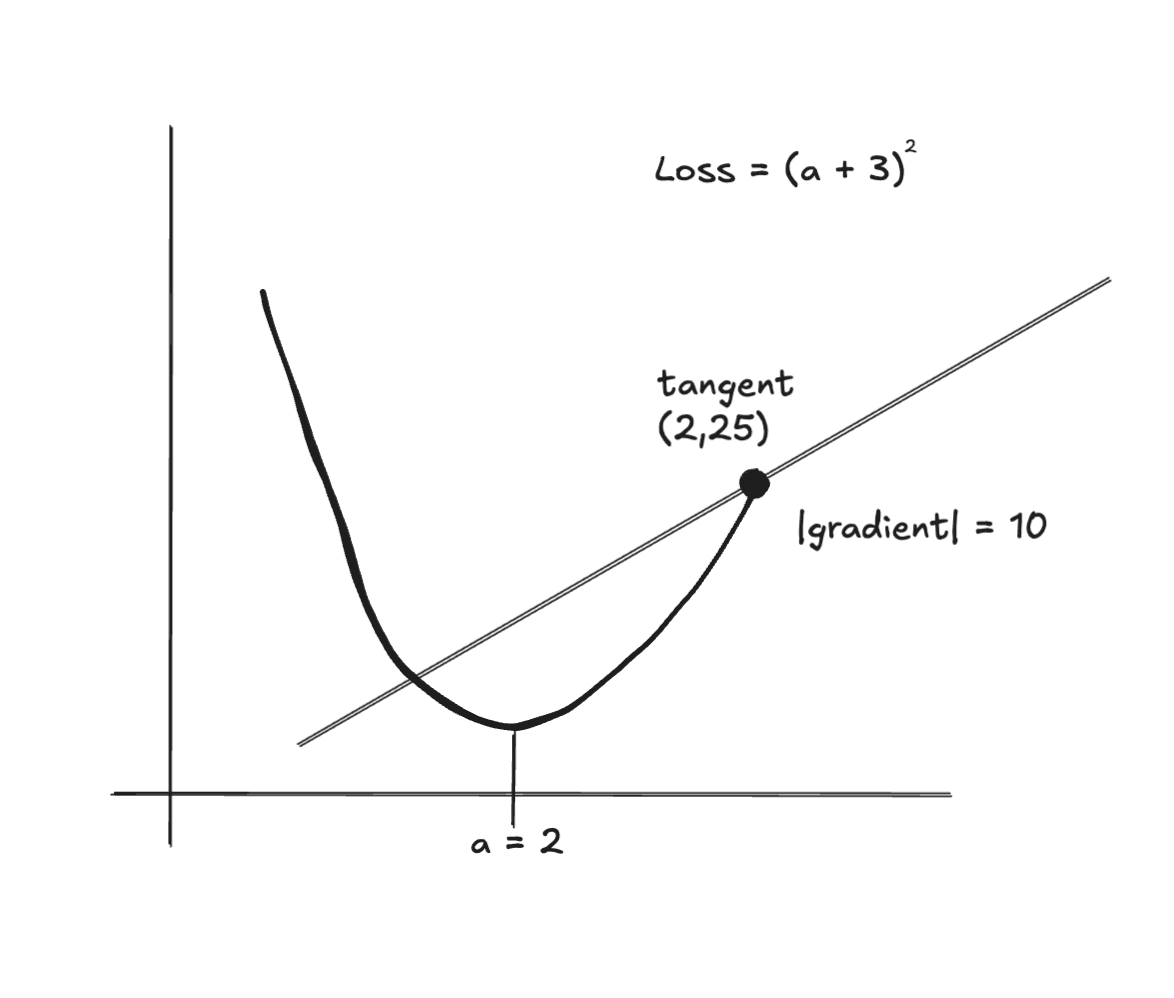
You can imagine a slider on a which as you move it from right to left, updates the curve and the slope of the tangent line (our gradient).

If we update a to 5, then our loss goes from 25 to 64. And our loss gradient with respect to a goes from 10 to 16.

We can repeat the same process for b:

∂c/∂b = 1  (if you increase b by 1, c increases by 1)
∂Loss/∂b = ∂Loss/∂c × ∂c/∂b = 10 × 1 = 10

Okay, now that we’re good on the chain rule, let’s define our add function.

impl Tensor {

// previous functions

pub fn add(self, other: &Tensor) -> Tensor {
// compute forward pass data operation
let data = self.data() + other.data();

// create clones of the data that we can hand off to our backward_fn
let self_clone = self.clone();
let other_clone = other.clone();

// create the output tensor first and we'll fill in the backward_fn next
let output = Tensor::from_op(data, vec![self.clone(), other.clone()], Box::new(|| {}));

// clone output for backward function
let output_clone = output.clone();

// define the backward func and box it on the heap to run later
let backward_fn = Box::new(move || {
// gradient from output (c)
let output_grad = output_clone.grad();

// use += to accumulate bc we might run this multiple times
self_clone.inner.lock().unwrap().grad += output_grad * 1.0;
other_clone.inner.lock().unwrap().grad += output_grad * 1.0;
});

// update the backward func
output.inner.lock().unwrap().backward_fn = Some(backward_fn);

output
}

}

Let’s walk through this step by step.

First, we add our tensors by adding the data fields of the two input tensors. Then we create clones of those tensors so that we can hand off ownership to the backward pass inside of the move closure (this is Rust after all!).

Then we create a stubbed output tensor. Why? Well in our backward pass, we need access to the output’s gradient (think of it like c from the chain rule example), so that we can add it to the our two input tensors (a and b from our chain rule example).

Also, notice that we use += the output_grad. A tensor might be used severasl times in which case we need to accumulate all of the gradients.

Then, we then add our backward_fn to our output tensor and then return it.

Lastly, we’re using .clone() a lot and we haven’t defined that trait, so let’s define it:

impl Clone for Tensor {
fn clone(&self) -> Tensor {
Tensor {
inner: Arc::clone(&self.inner),
}
}
}

Nothing too fancy here, just cloning our TensorData.

But wait! We can make this a little cleaner with a slight refactor. We’re already creating a new tensor in the from_op() function, so what if we just use that as our return tensor? Then we can get rid of of the output tensor we are creating in the add() function.

Here are the updates:

// old
type BackwardFn = Box<dyn Fn() + Send>;

// new takes gradient as param
type BackwardFn = Box<dyn Fn(f64) + Send>;

No change needed to the from_op() function and here is the updated add() function:

pub fn add(&self, other: &Tensor) -> Tensor {
// compute forward pass data operation
let data = self.data() + other.data();

// create clones of the data that we can hand off to our backward_fn
let self_clone = self.clone();
let other_clone = other.clone();

// define the backward func and box it on the heap to run later
let backward_fn = Box::new(move |grad_output: f64| {
// use += to accumulate bc we might run this multiple times
self_clone.inner.lock().unwrap().grad += grad_output * 1.0;
other_clone.inner.lock().unwrap().grad += grad_output * 1.0;
});

let prev = vec![self.clone(), other.clone()];

Tensor::from_op(data, prev, backward_fn)
}

We removed the output tensor we created and just passed in the gradient to the BackwardFn. We also now pass in a reference to self in the add() function signature so we can borrow it.

Much cleaner. Let’s test it and compare it with Pytorch.

use nanograd::tensor::Tensor;

fn main() {
let a = Tensor::new(2.0);
let b = Tensor::new(3.0);
let c = a.add(&b);
let d = a.data() + b.data(); // same thing as above, just showing another option
println!("data: {}", c.data());
println!("data: {}", d);
}

Finished `dev` profile [unoptimized + debuginfo] target(s) in 0.30s
Running `target/debug/nanograd`
data: 5
data: 5

import torch

a = torch.tensor(2.0, requires_grad=True)
b = torch.tensor(3.0, requires_grad=True)
c = a + b
print(f"c: {c.item()}")

(nanograd-py) [11/8/25 11:31:47] ~/code/projects/nanograd-py (main ✗) uv run main.py
c: 5.0

Nice! Things are looking good. We can now add our tensors and do a very simple forward pass. Time to build on it.

Multiplication

We’ve already laid the foundation for the multiplication operation with the work we did above on the addition operation. So let’s make a few updates and create a multiplication operation.

When we do c = a * b:

• Forward: c = a × b

• Backward:

• ∂c/∂a = b (if you increase a, c changes by b)

• ∂c/∂b = a (if you increase b, c changes by a)

So:

• ∂Loss/∂a = ∂Loss/∂c × b
• ∂Loss/∂b = ∂Loss/∂c × a

Let’s write the code for it:

pub fn mul(&self, other: &Tensor) -> Tensor {
let data = self.data() * other.data();

let self_clone = self.clone();
let other_clone = other.clone();

let backward_fn = Box::new(move |grad_output: f64| {
self_clone.inner.lock().unwrap().grad += grad_output * other_clone.data();
other_clone.inner.lock().unwrap().grad += grad_output * self_clone.data();
});

let prev = vec![self.clone(), other.clone()];

Tensor::from_op(data, prev, backward_fn)
}

One thing to note is that in the addition operation we multipled the grad_output by 1.0 (also called the local gradient) since ∂c/∂a = 1 and ∂c/∂b = 1 but in the multiplication operation we’re actually multiply it by the original data values.

Why do we do this?

In addition, the derivatives are constants. If you increase a by 1, you increase c by 1. However, in multiplication, the derivative is:

• ∂c/∂a = b (depends on b)
• ∂c/∂b = a (depends on a)

So if b = 10, then increasing a by 1 increases c by 10. But if b = 100, increasing a by 1 increases c by 100!

Let’s test our implementation against Pytorch:

use nanograd::tensor::Tensor;

fn main() {
let a = Tensor::new(2.0);
let b = Tensor::new(3.0);
let c = a.mul(&b);
println!("data: {}", c.data());
}

Finished `dev` profile [unoptimized + debuginfo] target(s) in 0.17s
Running `target/debug/nanograd`
data: 6

import torch

a = torch.tensor(2.0, requires_grad=True)
b = torch.tensor(3.0, requires_grad=True)
c = a * b
print(f"c: {c.item()}")

(nanograd-py) [11/9/25 8:25:04] ~/code/projects/nanograd-py (main ✗) uv run main.py
c: 6.0

Power

Last operation for now, let’s do powers. This is usefulf for things like MSE (mean squared error) which is often used in loss functions. Let’s lay out the forward and backward pass like we did above:

When c = a^n:

• Forward: c = a^n
• Backward: ∂c/∂a = n × a^(n-1)

So: ∂Loss/∂a = ∂Loss/∂c × n × a^(n-1)

The power operation is different from the other two in that there is no other tensor, it’s just one tensor being raised to a power. Let’s see the code:

pub fn pow(&self, n: f64) -> Tensor {
let data = self.data().powf(n);

let self_clone = self.clone();

let backward_fn = Box::new(move |grad_output: f64| {
self_clone.inner.lock().unwrap().grad +=
grad_output * n * self_clone.data().powf(n - 1.0);
});

let prev = vec![self.clone()];

Tensor::from_op(data, prev, backward_fn)
}

And let’s test it against Pytorch:

use nanograd::tensor::Tensor;

fn main() {
let a = Tensor::new(3.0);
let b = a.pow(2.0);
println!("data: {}", b.data());
}

Finished `dev` profile [unoptimized + debuginfo] target(s) in 0.20s
Running `target/debug/nanograd`
data: 9

import torch

a = torch.tensor(3.0, requires_grad=True)
b = a**2
print(f"b: {b.item()}")  # 9.0

(nanograd-py) [11/9/25 8:37:18] ~/code/projects/nanograd-py (main ✗) uv run main.py
b: 9.0

Nice! We’re getting pretty good at this. And with that, phase 2 is now complete! We now have our core data structures, computional graph and forward pass operations.

Onto phase 3!

Implementing Backward Pass

This is where we make nanograd actually work. We need to implement a backward pass function that:

1. Traverses the computation graph in reverse topological order
2. Calls each node’s backward function
3. Propagates gradients from output to inputs

Let’s start with an example:

let a = Tensor::new(2.0);
let b = Tensor::new(3.0);
let c = a.mul(&b);      // c = 6
let d = c.add(&a);      // d = 8
let loss = d.pow(2.0);  // loss = 64

The computational graph looks like this:

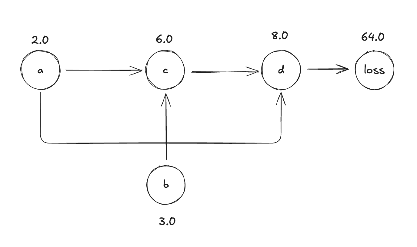
The forward order: a, b → c → d → loss

The backward order (reverse topological): loss -> d -> c -> a, b

We need to visit nodes so that when we process a node, all nodes that depend on it have already been processed. Let’s sketch out the algorithm before we implement it:

1. Start at the output node (loss)
2. Set loss.grad = 1.0 (seed gradient)
3. Build topological order (DFS)
4. For each node in reverse topological order:
- If it has a backward_fn:
- Call backward_fn(node.grad)
- This updates the gradients of parent nodes

First things first, we need to write a helper function that can build the reverse topological order. Let’s stub it out:

fn build_reverse_top_order(&self) -> Vec<Tensor> {
// the vec that we return
let mut topo = Vec::new();
// stores the nodes that we have already visited
let mut visited = HashSet::new();

fn build_reverse_top_order_recursive(
tensor: &Tensor,
topo: &mut Vec<Tensor>,
visited: &mut HashSet<>,
) {

//implement here

}
}

We’re creating a function to build the order and inside of that function, writing another function that we will call recursively to iterate over our nodes.

Inside of the recursive function, we need some way to identify unique tensors so that we can check in our hashset if we have already visited it. What can we use? Well, we can’t use the data, gradients or parents because those aren’t guaranteed to be unique. What about an Arc pointer? Yes! we’ll always have a unique pointer so we can use the pointer value itself as a unique way of identifying the tensor.

Let’s update our function:

fn build_reverse_top_order(&self) -> Vec<Tensor> {
// the vec that we return
let mut topo = Vec::new();
// stores the nodes that we have already visited
let mut visited = HashSet::new();

fn build_reverse_top_order_recursive(
tensor: &Tensor,
topo: &mut Vec<Tensor>,
visited: &mut HashSet<*const ()>,
) {
// create a unique pointer for this tensor
let ptr = Arc::as_ptr(&tensor.inner) as *const ();


// if we have seen this tensor before then we can just return
if visited.contains(&ptr) {
return;
}
// insert into the hashset so we can mark that we visisted it
visited.insert(ptr);

// finish implementation here
}
}

What’s happening here? We’re creating a hashset of pointers to our tensors that are allocated on the heap and using that pointer as a unique value to tell if we’ve already visited that tensor as we build the reverse topological order.

Let’s finish up the implementation:

fn build_reverse_top_order(&self) -> Vec<Tensor> {
// the vec that we return
let mut topo = Vec::new();
// stores the nodes that we have already visited
let mut visited = HashSet::new();

fn build_reverse_top_order_recursive(
tensor: &Tensor,
topo: &mut Vec<Tensor>,
visited: &mut HashSet<*const ()>,
) {
// create a unique pointer for this tensor
let ptr = Arc::as_ptr(&tensor.inner) as *const ();

if visited.contains(&ptr) {
return;
}

visited.insert(ptr);

let prev_unwrapped = tensor.inner.lock().unwrap().prev.clone();

for parent in prev_unwrapped.iter() {
build_reverse_top_order_recursive(parent, topo, visited);
}
// Add current node after all parents
topo.push(tensor.clone());
}
build_reverse_top_order_recursive(self, &mut topo, &mut visited);
topo
}

Next, we lock the tensor (since it’s meant to be thread-safe) and then we access the prev vector of tensors which are the parents. We create a clone so we don’t run into ownership problems later on.

Then we recursively iterate over the parents in the prev vector and push the input tensor to the topo vector to build the order.

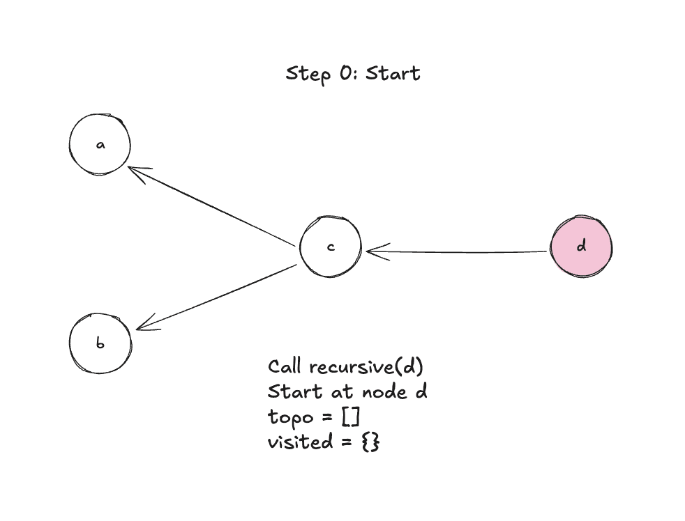
Let’s walk through it step-by-step:

Step 0: Function start, call recursive(d)

Step 1: Mark d as visited, visit it’s parents

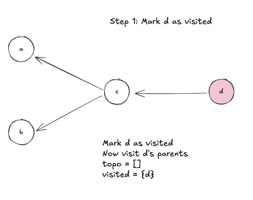
Step 2: Visit parent c

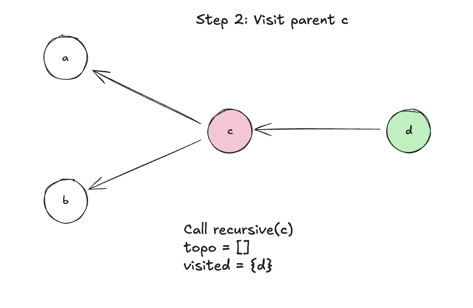
Step 3: Mark c as visited

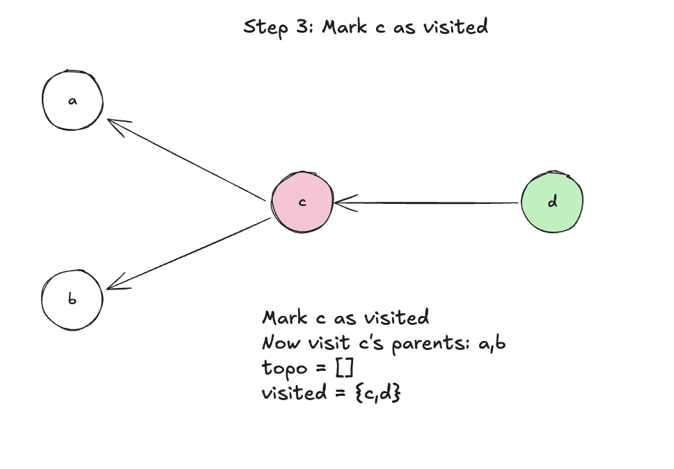
Step 4: Visit parent a

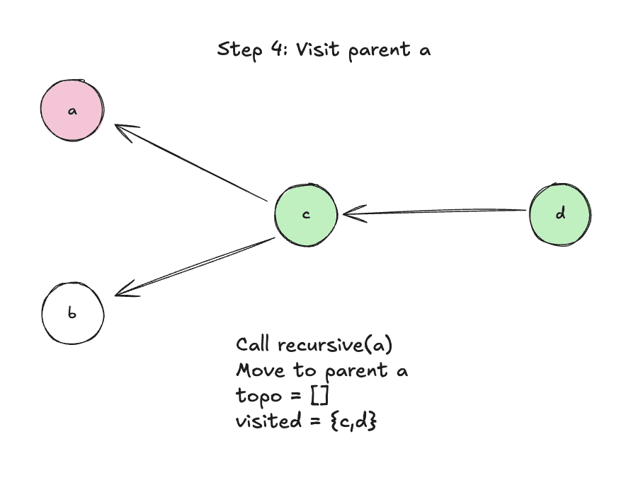
Step 5: Add a to topo since it has no parents

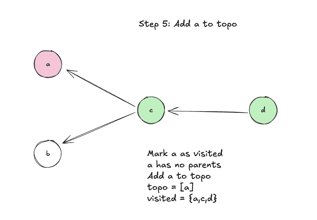
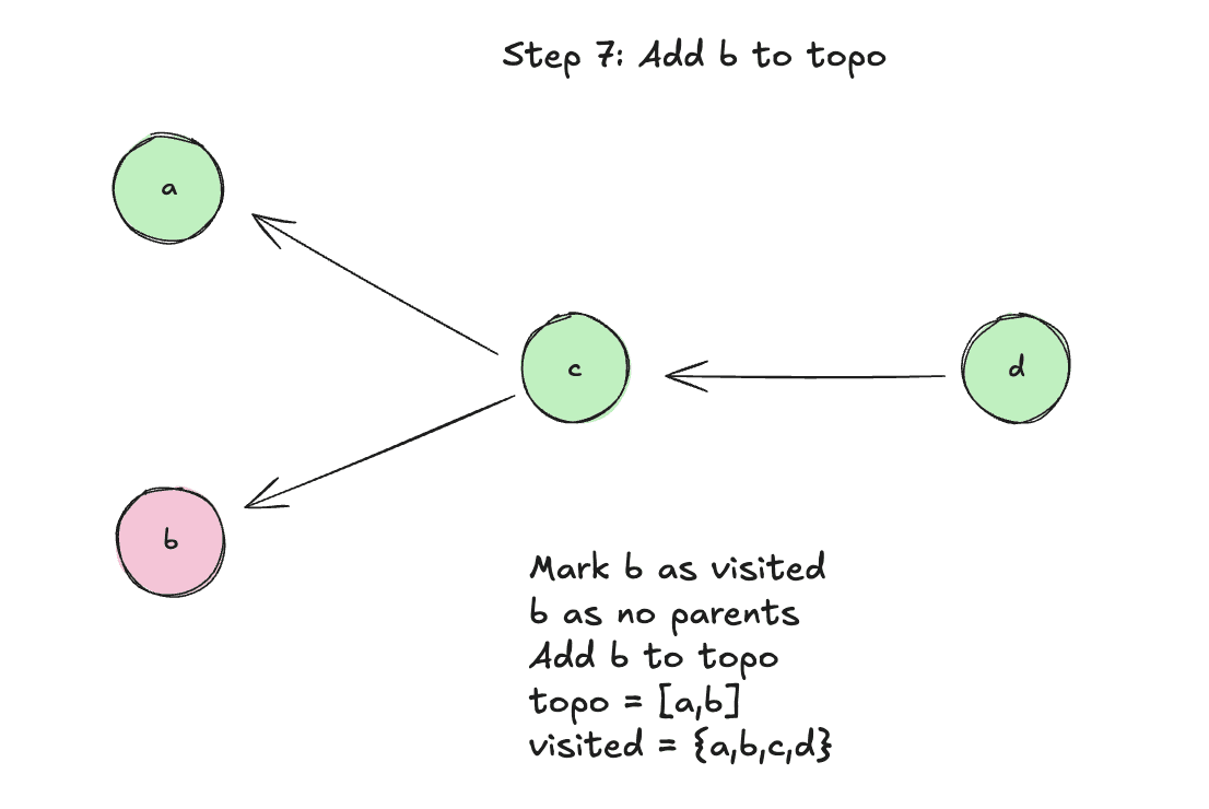
Step 6: Visit parent b

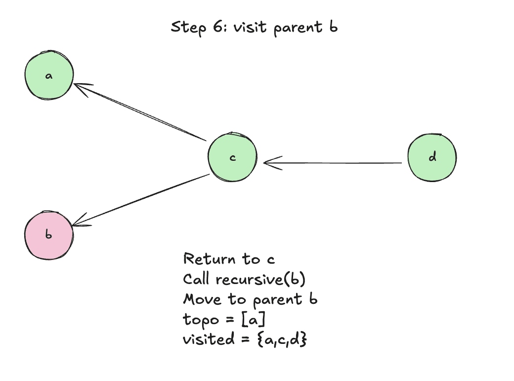
Step 7: Add b to topo

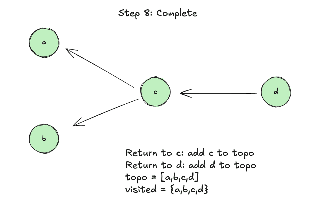
Step 8: Complete

Nice! To be honest, that took me longer than I want to admit to get right, so if you need to read it more than once, it’s totally fine (at least tell me that so I can feel better).

Okay, now we’re onto the last part: writing the backward pass function to bring all of this together.

Here’s what we need to do:

1. Build the topological order
2. Set this tensor’s gradient to 1.0 (seed the gradient)
3. Go through each tensor in reverse order
4. Call its backward function (if it has one)

Let’s see the code:

pub fn backward(&self) {
let topo = self.build_reverse_top_order();

self.inner.lock().unwrap().grad = 1.0;

for tensor in topo.iter().rev() {
let grad = tensor.grad();

let should_call = tensor.inner.lock().unwrap().backward_fn.is_some();

if should_call {
if let Some(ref func) = tensor.inner.lock().unwrap().backward_fn {
func(grad);
}
}
}
}

Like we outlined in our steps, we first build our order using our helper functions. Then we initially seed the gradient by setting it to 1.0. Then we loop over the order and for each tensor, get the gradient, check to see if it has a backward_fn and if it does, call it and pass in our gradient value.

Remember from our operations above, for example the addition operation, we defined the backward function to just take in an f64 gradient:

let backward_fn = Box::new(move |grad_output: f64| {
// use += to accumulate bc we might run this multiple times
self_clone.inner.lock().unwrap().grad += grad_output * 1.0;
other_clone.inner.lock().unwrap().grad += grad_output * 1.0;
});

Let’s test it using the multiplication operation:

use nanograd::tensor::Tensor;

fn main() {
let a = Tensor::new(2.0);
let b = Tensor::new(3.0);
let c = a.mul(&b); // c = 6.0

c.backward();

println!("a.grad: {}", a.grad());
println!("b.grad: {}", b.grad());
}

[11/10/25 9:39:44] ~/code/projects/nanograd (main ✗) cargo run
Compiling nanograd v0.1.0 (/Users/evisdrenova/code/projects/nanograd)
Finished `dev` profile [unoptimized + debuginfo] target(s) in 0.10s
Running `target/debug/nanograd`
a.grad: 3
b.grad: 2

import torch

a = torch.tensor(2.0, requires_grad=True)
b = torch.tensor(3.0, requires_grad=True)
c = a * b  # c = 6.0

c.backward()

print(f"a.grad: {a.grad.item()}")  # Should be 3.0
print(f"b.grad: {b.grad.item()}")  # Should be 2.0

(nanograd-py) [11/10/25 9:39:08] ~/code/projects/nanograd-py (main ✗) uv run main.py
a.grad: 3.0
b.grad: 2.0

Things are looking good. Let’s do one more test, a complicated one to really put our work to the test.

use nanograd::tensor::Tensor;

fn main() {
let a = Tensor::new(2.0);
let b = Tensor::new(3.0);
let c = a.mul(&b); // c = 6.0
let d = c.add(&a); // d = 8.0
let e = d.pow(2.0); // e = 64.0

e.backward();

println!("e.data: {}", e.data());
println!("e.grad: {}", e.grad());
println!("d.grad: {}", d.grad());
println!("c.grad: {}", c.grad());
println!("a.grad: {}", a.grad());
println!("b.grad: {}", b.grad());
}

[11/10/25 9:42:31] ~/code/projects/nanograd (main ✗) cargo run
Compiling nanograd v0.1.0 (/Users/evisdrenova/code/projects/nanograd)
Finished `dev` profile [unoptimized + debuginfo] target(s) in 0.09s
Running `target/debug/nanograd`
e.data: 64
e.grad: 1
d.grad: 16
c.grad: 16
a.grad: 64
b.grad: 32

import torch

a = torch.tensor(2.0, requires_grad=True)
b = torch.tensor(3.0, requires_grad=True)
c = a * b  # c = 6.0
d = c + a  # d = 8.0
e = d**2  # e = 64.0

e.backward()

print(f"e: {e.item()}")
print(f"a.grad: {a.grad.item()}")  # Should be 64.0
print(f"b.grad: {b.grad.item()}")  # Should be 32.0

(nanograd-py) [11/10/25 9:42:44] ~/code/projects/nanograd-py (main ✗) uv run main.py
e: 64.0
a.grad: 64.0
b.grad: 32.0

We’re in business!

Let’s take a second and summarize what we did here with the backward pass.

1. Topo order: [a, b, c, d, e] (leaves to root)
2. Reverse topo: [e, d, c, b, a] (root to leaves) ← This is what we iterate through with for tensor in topo.iter().rev(){}
3. Seed gradient at e: e.grad = 1.0 ← In a real model, we would calculate this in the forward pass
4. Process e: Call e.backward_fn(1.0) → updates d.grad
5. Process d: Call d.backward_fn(d.grad) → updates c.grad and a.grad
6. Process c: Call c.backward_fn(c.grad) → updates a.grad and b.grad
7. Process b: No backward_fn (leaf), skip
8. Process a: No backward_fn (leaf), skip

We start the root and seed it with grad = 1.0. Then we go through the order in reverse, with each node’s backward_fn updates its parents’ gradients. Remember that the parents are to the left of the nodes when we go backwards.

Lastly, we accumulate the gradients at the leafs. So a gets gradient from both c and d (they both use a; remember composite functions), so we use +=. The same is true for b.

The gradient tells us: “If I change a by a tiny bit, how much does e (the loss) change?”

Adding Non-linearity

So far we’ve built the core blocks of the nanograd system and we’re almost ready to put it all together in a training loop. Before we do that, we have to add in just one more operations: ReLU. This is a non-linear activation functions which give our neural nets the ability to truly learn. I wrote a blog on activation functions if you want to do a little more reading.

ReLU

ReLU is super simple: ReLU(x) = max(0, x)

Forward: If x > 0, output x. Otherwise output 0.

Backward:

• If x > 0: gradient passes through (multiply by 1)
• If x ≤ 0: gradient is blocked (multiply by 0)

Mathematically: ∂ReLU/∂x = 1 if x > 0 else 0

Here’s the code:

pub fn relu(&self) -> Tensor {
let data = if self.data() > 0.0 { self.data() } else { 0.0 };

let self_clone = self.clone();

let backward_fn = Box::new(move |grad_output: f64| {
let local_grad = if self_clone.data() > 0.0 { 1.0 } else { 0.0 };

self_clone.inner.lock().unwrap().grad += grad_output * local_grad;
});

Tensor::from_op(data, vec![self.clone()], backward_fn)
}

In the forward pass, we just check if the data is greater than 0, if so, then we pass it through otherwise we return a 0. We do something similar in the backward_fn. We pass in the gradient and then update the gradient on the original tensor.

Let’s do a test with Pytorch and verify:

use nanograd::tensor::Tensor;

fn main() {
let a = Tensor::new(3.0);
let b = a.relu();
b.backward();

assert_eq!(b.data(), 3.0); // 3.0 stays 3.0
assert_eq!(a.grad(), 1.0); // Gradient passes through

let a = Tensor::new(-3.0);
let b = a.relu();
b.backward();

assert_eq!(b.data(), 0.0); // -3.0 becomes 0.0
assert_eq!(a.grad(), 0.0); // Gradient blocked
}

[11/10/25 10:12:36] ~/code/projects/nanograd (main ✗) cargo run
Compiling nanograd v0.1.0 (/Users/evisdrenova/code/projects/nanograd)
Finished `dev` profile [unoptimized + debuginfo] target(s) in 0.21s
Running `target/debug/nanograd`

The no return value means that it was true.

import torch
import torch.nn.functional as F

a = torch.tensor(3.0, requires_grad=True)
b = F.relu(a)
b.backward()
print(f"b: {b.item()}, a.grad: {a.grad.item()}")

a = torch.tensor(-3.0, requires_grad=True)
b = F.relu(a)
b.backward()
print(f"b: {b.item()}, a.grad: {a.grad.item()}")

(nanograd-py) [11/10/25 9:43:28] ~/code/projects/nanograd-py (main ✗) uv run main.py
b: 3.0, a.grad: 1.0
b: 0.0, a.grad: 0.0

ReLU is done! Now we are ready. We are finally ready to build a neural net.

Onto step 5!

Building a Neural net

We’re going to build a simple neural net from the ground up.

The foundational building block of a neural net is the Neuron.

Neurons have:

1. Weights (one per input)
2. Bias
3. Computes output = relu(w₁×x₁ + w₂×x₂ + ... + wₙ×xₙ + b)

For example, a Neuron with three inputs:

inputs: [x₁, x₂, x₃]
weights: [w₁, w₂, w₃]
bias: b

output = relu(w₁×x₁ + w₂×x₂ + w₃×x₃ + b)

Let’s create a new file called src/neuron.rs for our Neuron implementation.

Next, let’s create the Neuron struct:

pub struct Neuron {
weights: Vec<Tensor>,
bias: Tensor,
is_output: bool,
}

The neuron will have a weights field that is a vector of Tensors, a bias field which is just a tensor and then an is_output field which we will use to determine if we should multiply by the activation function. We only want to do that in hidden layers and not output layers.

Next, let’s define the Neuron implementation:

use crate::tensor::Tensor;
use rand::Rng;

pub struct Neuron {
weights: Vec<Tensor>,
bias: Tensor,
}

impl Neuron {
pub fn new(num_inputs: usize) -> Self {
let mut rng = rand::rng();

// Initialize weights randomly between -1 and 1
let weights = (0..num_inputs)
.map(|_| Tensor::new(rng.random_range(-1.0..1.0)))
.collect();

// Initialize bias to 0
let bias = Tensor::new(0.0);

Neuron {
weights,
bias,
is_output,
}
}

}

First, we have to add in the rand crate with cargo add rand. Then we created a method to intialize a new Neuron with the num_inputs arg which defines how many weights we want to randomly create. Then we return the newly created Neuron with random weights and no bias.

Next, let’s create the forward pass function which we defined in the output above.

impl Neuron {
//..
pub fn new(num_inputs: usize, is_output: bool) -> Self {
let mut sum = Tensor::new(0.0);

for i in 0..self.weights.len() {
sum = sum.add(&self.weights[i].mul(&inputs[i]));
}

sum = sum.add(&self.bias);

// only apply ReLU if NOT output neuron
if self.is_output {
sum // Linear output
} else {
sum.relu() // Hidden layers use ReLU
}
}
}

The forward pass function is a straight implementation of output = relu(w₁×x₁ + w₂×x₂ + ... + wₙ×xₙ + b). We initialize a new Tensor with data set to 0.0, then iterate over the weights and input multiplying them together at the same indices and then accumulating the sum. We add the bias and then call the relu() method if it’s not the output neuron.

While we’re at it, let’s also add in a function to easily get the parameters:

pub fn parameters(&self) -> Vec<Tensor> {
// return all parameters (weights + bias) for training
let mut params = self.weights.clone();
params.push(self.bias.clone());
params
}

This will come in handy later on.

Next, let’s create a Layer.

We then stack neurons to create a layer.

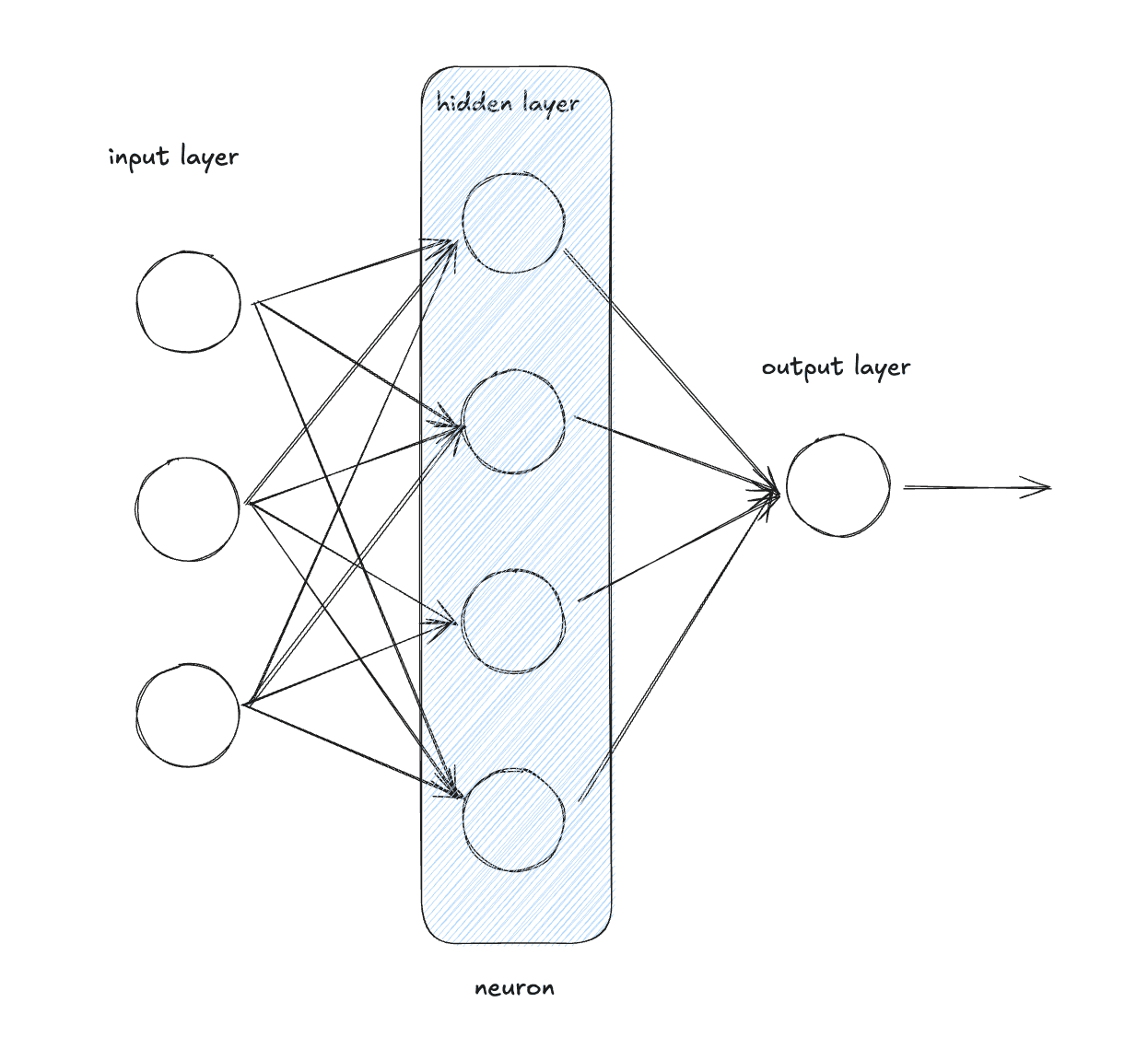
A layer is just a collection of Neurons. Each Neuron gets the same input and produces an output. Remember that Neurons are initialized with different random weights so the outputs will be different.

pub struct Layer {
neurons: Vec<Neuron>,
}

impl Layer {
pub fn new(num_inputs: usize, num_outputs: usize, is_output: bool) -> Self {
let neurons = (0..num_outputs)
.map(|_| Neuron::new(num_inputs, is_output))
.collect();

Layer { neurons }
}

}

We create a Layer struct that holds a vector of Neurons. Then we create a Layer implementation which has a method to initialize a new layer. The initialization creates a num_outputs number of Neurons in the Layer.

Let’s write the rest of the layer implementation:

impl Layer {

//...

pub fn forward(&self, inputs: &[Tensor]) -> Vec<Tensor> {
self.neurons
.iter()
.map(|neuron| neuron.forward(inputs))
.collect()
}

pub fn parameters(&self) -> Vec<Tensor> {
self.neurons
.iter()
.flat_map(|neuron| neuron.parameters())
.collect()
}
}

Like the Neuron implementation, we define a forward function and a paramter function. We’ve already done the hard work in the Neuron implementation, so here we’re just mapping over the Neurons and collecting the results into a vector and returning it.

Lastly, let’s create a multi-layer perceptron by stacking layers

The MLP implementation is going to be very very similar to the layer implementation so I’m just going to paste it here:

#[derive(Clone)]
pub struct MLP {
layers: Vec<Layer>,
}

impl MLP {
pub fn new(num_inputs: usize, layer_sizes: &[usize]) -> Self {
let mut layers = Vec::new();
let mut input_size = num_inputs;

for (i, &output_size) in layer_sizes.iter().enumerate() {
let is_last_layer = i == layer_sizes.len() - 1;
layers.push(Layer::new(input_size, output_size, is_last_layer));
input_size = output_size;
}

MLP { layers }
}

pub fn forward(&self, inputs: &[Tensor]) -> Vec<Tensor> {
let mut current = inputs.to_vec();

for layer in &self.layers {
current = layer.forward(&current);
}

current
}

pub fn parameters(&self) -> Vec<Tensor> {
self.layers
.iter()
.flat_map(|layer| layer.parameters())
.collect()
}
}

Alright, folks, we’ve finally reached the last part.

Let’s build the training loop.

Building a Training Loop

This is the last phase where we put everything together. There are three things that we need:

1. Loss function: we’ll use mean squared error (MSE) for this
2. Training data (a simple data set)
3. Training loop (forward pass, backward pass, update weights)

First, let’s add a way to update the parameters after computing the gradients. We can update our Tensor implementation by adding these two functions:

impl Tensor {
// ...

pub fn zero_grad(&self) {
self.inner.lock().unwrap().grad = 0.0;
}

pub fn update(&self, learning_rate: f64) {
let mut locked = self.inner.lock().unwrap();
locked.data -= learning_rate * locked.grad;
}
}

The zero_grad function is pretty straightforward, it just zeros out the gradient.

The update function updates the parameter by moving in the opposite direction of the gradient. The gradient tells us which direction the loss increases, so we subtract it to move toward lower loss. The learning rate controls how big of a step we take. multiplying it by the gradient scales the step size. So data -= learning_rate * grad means “move the parameter in the direction that reduces the loss, by a step of size learning_rate × gradient”.

First, we need to create our neural net. We can use our MLP implementation to define a neural net like this:

let mlp = MLP::new(2, &[8, 1]);

This creates a multi-layer perceptron neural net with:

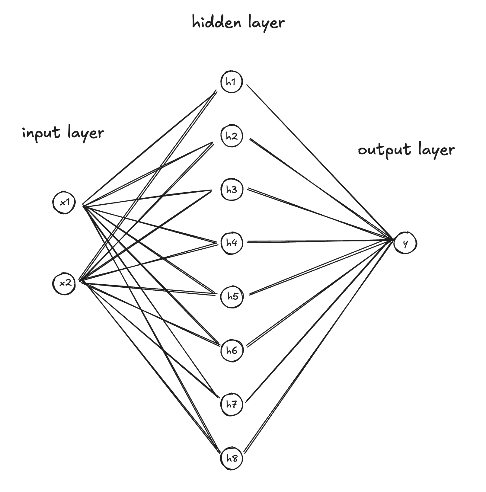
• Input: 2 values
• Layer 1: 2 inputs → 8 outputs (hidden layer with ReLU)
• Layer 2: 8 inputs → 1 output (output layer, no ReLU)

It has a total of 33 parameters. Slightly smaller than GPT4 at an estimated 1.7 Trillion parameters...

Now, we need a dataset. A classic data set to train basic neural nets is the XOR data set.

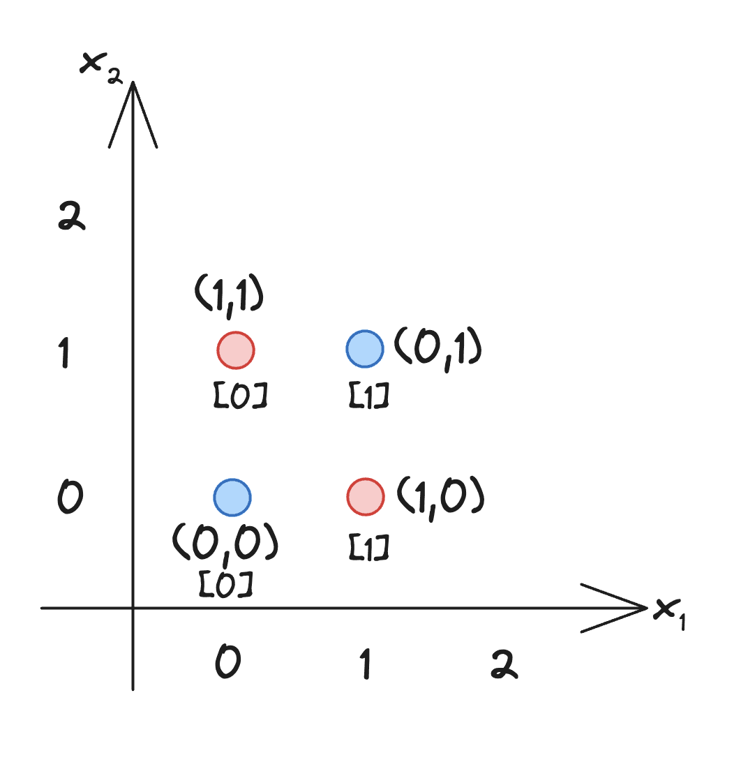
It’s not linearly seperable without a hidden layer meaning that you cannot draw a linear line on this coordinate plane in order to separate the red and blue dots. It requires a hidden layer.

// Simple dataset: XOR-like problem
// Input: [x1, x2], Target: x1 XOR x2
let dataset = vec![
(vec![0.0, 0.0], 0.0),
(vec![0.0, 1.0], 1.0),
(vec![1.0, 0.0], 1.0),
(vec![1.0, 1.0], 0.0),
];

Notice that the dataset is a vector of tuples where the first element of the tuple is the input data and the second element is the target data. In our training loop, we need to convert this dataset into our Tensor types. We can do that like this:

// Simple dataset: XOR-like problem
// Input: [x1, x2], Target: x1 XOR x2
let dataset = vec![
(vec![0.0, 0.0], 0.0),
(vec![0.0, 1.0], 1.0),
(vec![1.0, 0.0], 1.0),
(vec![1.0, 1.0], 0.0),
];

let tensor_dataset: Vec<(Vec<Tensor>, Tensor)> = dataset
.iter()
.map(|(inputs, target)| {
let tensor_inputs = inputs.iter().map(|&x| Tensor::new(x)).collect();

let tensor_target = Tensor::new(*target);

(tensor_inputs, tensor_target)
})
.collect();

Here we are iterating over the dataset and converting the input into a vector of tensors by looping over the input (since it’s a vector of f64s) and initializing a new Tensor for each element. The output is much easier, it’s just a single f64, so we can just initialize a new Tensor for that.

Nice, we have our data in the right shape. Now for the training loop.

The training loop needs to do the following for each epoch:

1. Zero gradients
2. Set the learning rate and the number of epochs
3. For each data point:

• Forward pass
• Compute loss (prediction - target)^2
• Backward pass

1. Update weights (using the update function we created earlier)
2. Print loss every 10 epochs

Let’s write the code:

let learning_rate = 0.05;
let epochs = 1000;

for epoch in 0..epochs {
// zero out gradients in between epoch runs
for j in mlp.parameters().iter() {
j.zero_grad();
}

// initialize loss
let mut total_loss = 0.0;

for (input, target) in &tensor_dataset {
// call forward pass
let prediction = mlp.forward(input);

// calc loss
let loss = prediction[0].sub(target).pow(2.0);
// calc gradients
loss.backward();

total_loss += loss.data();
}

// update weights
for param in mlp.parameters().iter() {
param.update(learning_rate);
}

if epoch % 50 == 0 {
let params = mlp.parameters();
let grad_sum: f64 = params.iter().map(|p| p.grad().abs()).sum();
println!(
"Epoch {}: Loss = {:.4}, Grad sum = {:.6}",
epoch, total_loss, grad_sum
);
}
}

We don’t have a substraction operation, but we can create a quick one using the inverse of our add operation and add it to our Tensor implementation:

pub fn sub(&self, other: &Tensor) -> Tensor {
// a - b = a + (-1 × b)
let neg_one = Tensor::new(-1.0);
self.add(&other.mul(&neg_one))
}

Let’s gve it a shot!

Here’s the entire training loop:

use nanograd::neuron::MLP;
use nanograd::tensor::Tensor;

fn main() {
let mlp = MLP::new(2, &[8, 1]);

let dataset = vec![
(vec![0.0, 0.0], 0.0),
(vec![0.0, 1.0], 1.0),
(vec![1.0, 0.0], 1.0),
(vec![1.0, 1.0], 0.0),
];

let tensor_dataset: Vec<(Vec<Tensor>, Tensor)> = dataset
.iter()
.map(|(inputs, target)| {
let tensor_inputs = inputs.iter().map(|&x| Tensor::new(x)).collect();

let tensor_target = Tensor::new(*target);

(tensor_inputs, tensor_target)
})
.collect();

let learning_rate = 0.05;
let epochs = 1000;

for epoch in 0..epochs {
// zero out gradients in between epoch runs
for j in mlp.parameters().iter() {
j.zero_grad();
}

// initialize loss
let mut total_loss = 0.0;

for (input, target) in &tensor_dataset {
// call forward pass
let prediction = mlp.forward(input);

// calc loss
let loss = prediction[0].sub(target).pow(2.0);

loss.backward();

total_loss += loss.data();
}

// update weights
for param in mlp.parameters().iter() {
param.update(learning_rate);
}

if epoch % 50 == 0 {
let params = mlp.parameters();
let grad_sum: f64 = params.iter().map(|p| p.grad().abs()).sum();
println!(
"Epoch {}: Loss = {:.4}, Grad sum = {:.6}",
epoch, total_loss, grad_sum
);
}
}

prin