October 15, 2025

Investment as a Source of Productivity Growth

Giuseppe Fiori, Colleen Lipa, William Wu1

1. Summary

Over the past two decades, the divergence in GDP per capita between the United States and major European economies has grown. Relative to 2000, this gap has widened to reach about 40 percent (see Panel A in Figure 1). This difference can be partially attributed to superior productivity performance in the U.S. economy compared to its European counterparts (see Figure 1 Panel B).2 This GDP per capita differential coincides with periods when the U.S. had higher growth in real equipment investment and invested in more efficient technologies (see Panels C and D in Figure 1).

Figure 1. GDP, Investment, and Productivity Measures

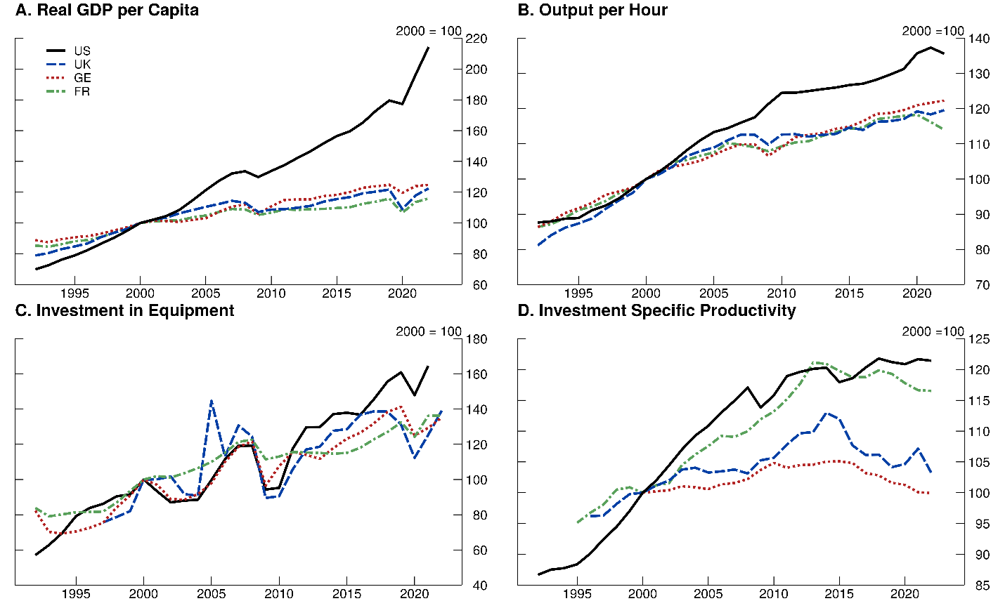
Note: All data are normalized to 100 in 2000. GDP per capita is measured in the domestic currency of each respective country. Investment-specific productivity is measured as the inverse of the relative price of investment, calculated using the CPI for nondurables, CPI for services, and the PPI for investment goods (see Appendix for full calculation details). Investment data are expressed in real terms.

Sources: WEO; OECD. See Appendix for further details.

Accessible version

In this note, we investigate the transmission mechanism through which capital accumulation enhances productivity, providing both firm-level empirical evidence that investment flows represent a significant contributor of long-run growth dynamics and a counterfactual analysis that demonstrates how European productivity would have evolved had the European countries had the same investment-specific productivity growth as the U.S.

In our empirical analysis, we use firm-level data to show that investment patterns are critical determinants of firm-level productivity across advanced economies. We demonstrate two key results: (1) firms with longer intervals since their last major capital adjustment exhibit systematically lower total factor productivity and (2) this relationship holds consistently across firms in the U.S., U.K., France, and Germany.

Our quantitative analysis shows that the U.S. invests in goods that embody superior productivity growth, which partially explains its productivity advantage. The differential investment rates and the quality associated with equipment investment account for approximately 55 percent of the observed productivity gap between these advanced economies, highlighting the critical role of capital formation in explaining cross-country growth differentials. The results suggest that slower technology adoption in investment goods in European economies is a large factor in its productivity performance relative to the U.S.

2. Investment Age and Productivity: Cross-Country Evidence

Investment in new equipment contributes to productivity growth by incorporating the latest, more efficient technologies into the production process; see, for instance, Solow (1960) and Greenwood et al. (1997). We use firm-level data from the U.S., U.K., France, and Germany to see how investment in capital affects total factor productivity.

2.1 Key Variables in the Empirical Framework Our analysis employs three core variables constructed from comprehensive firm-level datasets. First, we proxy the level of technology operated by the firm using investment age, the time elapsed since a firm’s last investment spike, defined as an annual investment rate exceeding 20 percent. This variable serves as a proxy for the technological vintage of the firm’s capital stock, following Power (1998) and Fiori and Scoccianti (2021 and 2024). Second, we calculate firm-level total factor productivity (TFP) from production function residuals, capturing the firm-specific efficiency component. Third, we incorporate the relative price of investment equipment to measure the technological frontier evolution.

We utilize firm-level data from Compustat for the U.S. (1972-2024) and CIQ Pro for European countries — U.K., France, and Germany (1990-2023) — following Bloom (2009)’s methodology for constructing capital accumulation and productivity measures.

2.1.1 Investment Age as a Technology Proxy Investment age captures the technological vintage available to firms based on the premise that major capital adjustments coincide with technology adoption. A firm’s investment age equals zero during investment spike years (investment rate ≥ 20 percent) and increases by one in subsequent years.3 Fiori and Scoccianti (2024) validate this approach using Italian data, showing that firms self-reporting outdated technology exhibit higher investment age.

Table 1 reveals that, on average, U.S. firms invest more than their European counterparts, whether we examine the average or median investment rate. Strikingly, the average investment age, the time elapsed between investment spikes, and the yearly share of firms are similar across countries, indicating similar investment cycles. Importantly, more firms in the U.S. experience investment spikes, indicating that U.S. firms are more likely to undertake large investment episodes and likely introduce newer technologies.

Table 1: Summary Statistics

U.S. U.K. France Germany Average Investment Rate 11% 3% 4% 5% Median Investment Rate 2% 0.60% 0.50% 0.90% Average Investment Age 3.65 3.3 3.63 3.75 Share of All Data with a Spike 21.11% 22.73% 19.78% 20.32% Share of Firms with a Spike 60.65% 52.94% 43.89% 42.45% Sample Period 1964-2024 1990-2023 1990-2023 1990-2023 Data Source Compustat CIQ North America CIQ Pro CIQ Pro CIQ Pro

Note: The average investment age and average investment rate are calculated by taking the mean of the investment age and investment rate across each country’s data. The median investment rate is the median value across each country’s data. A spike is calculated when the Investment Age = 0 and when the Investment rate is ≥ 20 percent The share of all data with a spike is how many spikes occur in the entire dataset. The share of firms with a spike is how many of the firms that are in the dataset experience a spike at least once.

Source: Compustat CIQ North America; CIQ Pro.

2.1.2 Firm-Level TFP Measurement We estimate firm-specific total factor productivity from the production function:

$$$$log{\left(y_{i,t}\right)}=\mu_i+\alpha_{k_s}log{\left(k_{i,t-1}\right)}+\alpha_{n_s}log{\left(n_{i,t}\right)}+\varepsilon_{i,t}\ (1)$$$$

where $$y_{i,t}$$ represents real sales, $$k_{i,t-1}$$ is the constructed capital stock following Bloom (2009), $$n_{i,t}$$ denotes employment, and $$\mu_i$$ captures firm, year, and sector fixed effects.

Using the coefficients of constructed capital stock and employment, we calculate our TFP measure from:

$$$$TFP_{i,t}=\log{\left(y_{i,t}\right)}-\alpha_{k_s}\log{\left(k_{i,t-1}\right)}-\alpha_{n_s}\log{\left(n_{i,t}\right)}\ (2)$$$$

We find substantial firm-level productivity heterogeneity, consistent with Syverson (2011). Detailed construction procedures are provided in the Appendix.

2.2 Empirical Results: Investment Age and Productivity To establish the relationship between investment age, the timing of large investment episodes, and productivity, we follow the approach in Power (1998) and estimate:

$$$$\log{\left(TFP_{i,t}\right)}=\beta\times{\mathrm{Inv.Age}}_{i,t-1}+\rho\times\log{\left(TFP_{i,t-1}\right)}+\mu+\varepsilon_{i,t}\ (3)$$$$

where $$\mu$$ include a comprehensive set of fixed effects (firm, sector, and year). This specification controls for productivity persistence while measuring the impact of investment age.

Table 2 presents consistently negative and statistically significant coefficients across all countries, confirming that delaying large investment episodes—and therefore delaying the introduction of newer technologies into production—predicts lower productivity.4 The economic magnitude is substantial: each additional year of investment age corresponds to a measurable productivity decline of about a third of a percent.

Table 2: Regression Results

Main Estimate	U.S.	U.K.	France	Germany
-0.459%**
-0.345%**
-0.241%*
-0.324%*

Note: We report the $$\beta$$ coefficient estimated from Equation 3 in the Main Estimate column. Significance is reported at the 1, 5, and 10 percent levels by ***, **, and *, respectively.

Source: FRB staff calculations using Compustat and CIQ Pro data.

These findings support the notion that investment timing represents a fundamental channel through which technological progress translates into firm-level productivity gains, with important implications for understanding cross-country productivity differentials.

In Figure 2 we show the cross-sectional distribution of investment age for every country considered in the empirical analysis. Based on the estimated negative correlation between investment age and firm’s TFP, we interpret the widespread heterogeneity in the timing of investment as a source of TFP heterogeneity across firms, with firms with newer capital displaying higher TFP than counterparts with older, less efficient, capital. This heterogeneity in investment behavior provides a natural setting for examining the productivity consequences of delayed capital adjustment across different institutional and economic environments. We turn to this issue next.

Figure 2. Proportion of Firm Investment Age

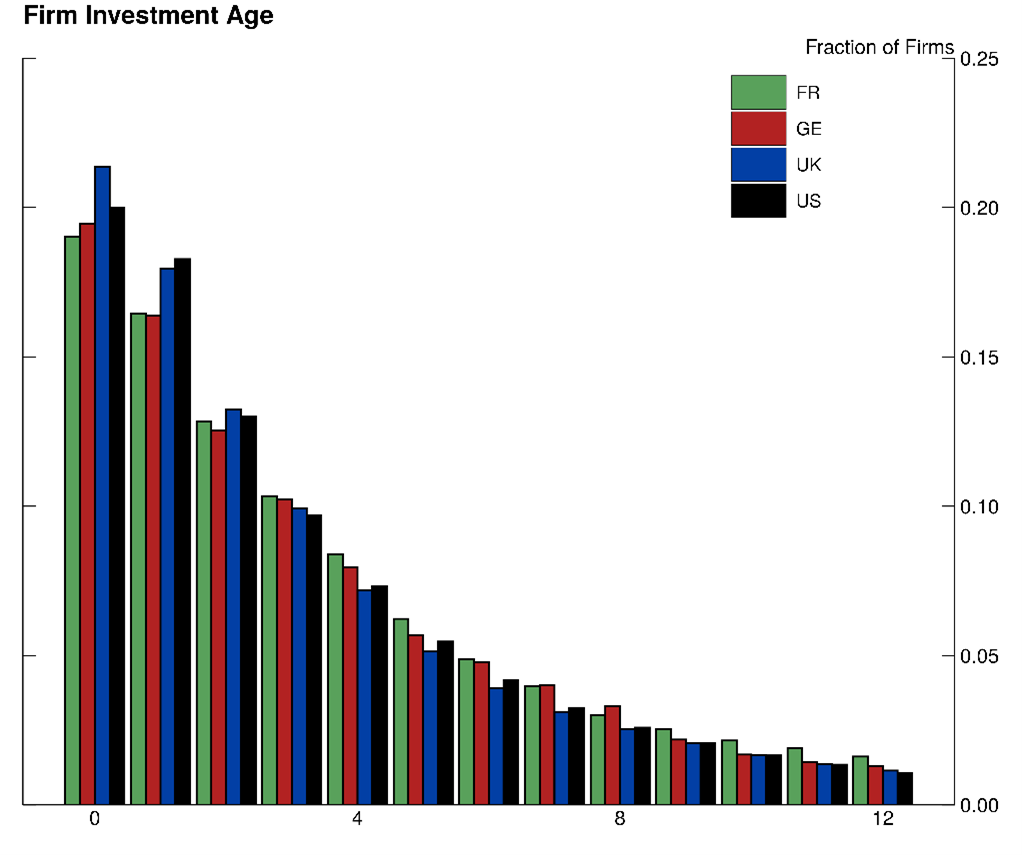
Note: This figure shows the fraction of all firms in the dataset for each country across their investment age. Key identifies in order from left to right. The green bars denote France, the red bars denote Germany, the blue bars denote the UK, and the black bars denote the U.S. All the countries follow the same pattern, with about 20 percent of the data having an investment age of 0.

Source: FRB staff calculations using Compustat and CIQ Pro data.

Accessible version

3. Investment Implications: A European Counterfactual

Having established that higher investment age systematically predicts lower total factor productivity, we now quantify the aggregate implications of these micro-level relationships. Specifically, we examine how much of the U.S.-Europe productivity gap can be attributed to differential investment-specific technological progress using a counterfactual analysis based on the framework of Greenwood et al. (1997), which decomposes output growth into contributions from capital deepening, labor, and investment-specific technological change.5

Our counterfactual asks: How would European productivity have evolved if these countries had experienced the same investment-specific productivity growth as the United States? The exercise proceeds in three steps. First, we calculate investment-specific productivity growth rates for the U.S. using relative equipment prices and investment data. Second, we replace each European country’s historical investment-specific productivity growth with the U.S. rate, holding all other factors constant. Third, we project counterfactual output per hour from 2000 through 2022, initializing each country with its actual 2000 productivity level. Detailed methodology and data construction procedures are provided in the Appendix.

Figure 3 presents the counterfactual trajectories alongside actual productivity paths for each European country, revealing substantial potential gains from faster investment-specific technological progress.

Figure 3. Counterfactual European Productivity with U.S. Investment-Specific Technology Growth

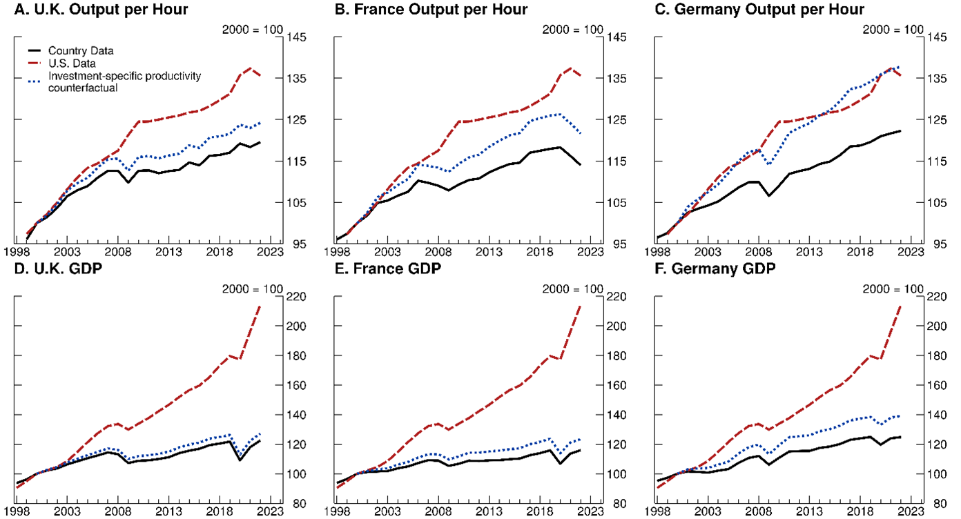
Note: These figures show the counterfactual results for the UK, France, and Germany. For each figure, the country data (solid black line) is the respective country’s Output per Hour and GDP data indexed to 2000. The US data (dashed red line) is the US’s Output per Hour and GDP indexed to 2000. The investment-specific productivity counterfactual (dotted blue line) is the respective country’s counterfactual Output per Hour and GDP calculated by the country’s investment in equipment and the US’s investment specific productivity.

Source: FRB staff calculations. See Appendix for further details.

Accessible version

The quantitative effects are economically significant. Had European countries experienced U.S. levels of investment-specific productivity growth beginning in 2000, the productivity gap with the United States would have been substantially smaller. Specifically, the relative output per hour gap would have been reduced by 29 percent for the United Kingdom, 35 percent for France, and 101 percent for Germany.6 The particularly large effect for Germany suggests that slower technology adoption in investment goods has been a critical factor in its productivity performance relative to the U.S. These findings indicate that investment-specific technological progress—the rate at which new technologies become embodied in capital goods—represents a quantitatively important source of cross-country productivity differentials.

This analysis abstracts from the potential gains from faster investment-specific technological progress, as it holds other factors constant. In particular, we do not account for potential general equilibrium effects whereby faster technological progress might alter firms’ investment behavior, factor prices, or the pace of creative destruction. Additionally, the framework assumes that European countries could have achieved U.S. rates of investment-specific productivity growth without addressing underlying institutional or structural differences that may have contributed to the observed gaps.7 Despite these limitations, the counterfactual exercise demonstrates that investment-specific technological change represents a quantitatively significant channel through which cross-country productivity differences emerge and persist over time.

4. Conclusion

Over the past two decades, rapid technology adoption and accelerated investment cycles have driven U.S. productivity and output growth far ahead of Europe. This divergence has only widened: while Europe’s average investment age continues to climb, the U.S. has begun renewing its capital stock at a faster pace. However, these differential capital accumulation patterns are themselves symptoms of deeper structural problems (Draghi, 2024). The productivity divergence between the United States and Europe fundamentally stems from deep-seated structural and regulatory differences that create systemic barriers to investment and innovation. As highlighted in the Draghi report, Europe suffers from a chronically fragmented Single Market with “differing authorization procedures and the large number of reporting authorities across the EU,” forcing innovative companies to seek US venture capital and expand in unified American markets rather than “tackling fragmented EU markets.” This regulatory fragmentation prevents European firms from accessing the scale economies and unified market conditions that enable American counterparts to rapidly deploy productivity-enhancing technologies, creating a structural disadvantage that perpetuates the widening economic divergence. Thus, while capital accumulation patterns explain much of the observed productivity gap, the underlying regulatory and institutional frameworks determine why European firms systematically underinvest in productivity-enhancing technologies compared to their American counterparts.

We find that investment patterns help determine productivity for firms in the U.S., U.K., France, and Germany and that the productivity gap is partially attributed to the U.S. having more investment in productive capital than its European counterparts, particularly at the technological frontier. As breakthrough technologies such as AI are being adopted in many different sectors of the economy, increases in investment by European firms will be even more important in reducing the output gap.

References

Bloom, Nicholas, “The Impact of Uncertainty Shocks,” Econometrica, May 2009, 77 (3), 623–685.

Cacciatore, Matteo, and Giuseppe Fiori (2016): “The Macroeconomic Effects of Goods and Labor Markets Deregulation,” Review of Economic Dynamics, 2016, 20, 1-24.

Cacciatore, Matteo, Giuseppe Fiori, and Fabio Ghironi (2016): “Market Deregulation and Optimal Monetary Policy in a Monetary Union,” Journal of International Economics, 99, 120–137.

Cavallo, Michele and Anthony Landry, “The Quantitative Role of Capital Goods Imports in US Growth,” American Economic Review, May 2010, 100 (2), 78–82.

Doms, Mark E. and Timothy Dunne, “Capital Adjustment Patterns in Manufacturing Plants,” Review of Economic Dynamics, April 1998, 1 (2), 409–429.

Draghi, Mario, “The Draghi report of EU competitiveness,” European Commission, 2024.

Fiori, Giuseppe, “Lumpiness, Capital Adjustment Costs and Investment Dynamics,” Journal of Monetary Economics, 2012, 59 (4), 381–392.

– and Filippo Scoccianti, “Aggregate Dynamics and Microeconomic Heterogeneity: The Role of Vintage Technology,” Bank of Italy Occasional Paper No. 651, 2021.

– and Filippo Scoccianti, “Aggregate Dynamics and Microeconomic Heterogeneity: The Role of Investment-Specific Technology,” working paper, 2024.

Greenwood, Jeremy, Zvi Hercowitz, and Per Krusell, “Long-Run Implications of Investment-Specific Technological Change,” American Economic Review, June 1997, 87 (3), 342–362.

Power, Laura, “The Missing Link: Technology, Investment, and Productivity,” The Review of Economics and Statistics, May 1998, 80 (2), 300–313.

Solow, Robert, Investment and Technological Progress, Stanford University Press, 1960.

Syverson, Chad, “What Determines Productivity?,” Journal of Economic Literature, June 2011, 49 (2), 326–65.

A. Cross-Country Evidence Analysis

A.1. Data Collection

A.1.1. United States The data for United States firms is collected from Compustat - Capital IQ - North America in the Fundamental Annual database. The data is collected from 1964-2024. The gvkey, Stock Exchange Code, Foreign Incorporation Code, SIC, Gross PPE, Net PPE, AQC, AT, SALE, EMP, and Cost of Goods Sold are collected. We use implicit price deflators for Personal Income from the NIPA Table 1.1.9 to get our nonresidential fixed investment good deflator.

A.1.2. France, Germany, United Kingdom Data for French, German, and English firms are gathered from CIQ Pro’s Company Screener. For each year from 1990-2023, the SIC; Property, Plant, and Equipment, Total Assets; Cost of Goods Sold; Total Revenue; and Total Employees is collected if the firm did not have any of these data missing. After this data is collected, the firm’s name, id, age, and Gross Property, Plant, and Equipment is also collected, though firms were kept if they were missing this data in a given year. We also obtain implicit price deflators, using OECD data on Private Final Consumption Expenditure Implicit Price Deflator for each respective country.

A.2. Data Cleaning We follow the methodology in Alfaro, Bloom and Lin (2024) to clean the firm level data. We remove utilities firms (SIC 4900 - 4999) because these are heavily regulated and therefore assumptions about cost minimization or profit maximization are unlikely to hold. We remove financial firms (SIC 6900 - 6999) because their balance sheets are much different from other firms. We only study firms who do business in U.S. Dollars (USD). We exclude observations with negative sales or employment. We additionally exclude observations that are missing data for employment, sales, and our calculated real net investment and real capital, as they cannot be used to calculate the variables in our regression. For the United States firms, we exclude observations where acquisitions are larger than 5 percent of the value of total assets. We were unable to collect an acquisitions variable for French, German, or English firms. We linearly interpolate to fill missing observations of PPENT, which is sometimes missing within a given firm’s investment spell. For each firm, we select the longest continuous fiscal year segment. If there are two segments that are equally as long, we select the segment that ends more recently.

A.3. Variable Creation

• **Real Capital Stock - **We calculate capital stock using the perpetual inventory method, using the first entry of PPEGT, the book value of capital stock, as our initial value.

$$$$k_{i,t}=\left(1-\delta\right)k_{i,t}-i_{i,t}$$$$

Afterwards, we deflate this using the investment goods deflator.

• Net Investment - We construct a measure of net investment.

$$$$i_{i,t}-\delta k_{i,t-1}=PPENT_{i,t}-PPENT_{i,t-1}$$$$

• Investment Rate - Following Bloom (2009), we define the investment rate for a given firm $$i$$ at time $$t$$ as

$$$$ik_{i,t}=\frac{i_{i,t}}{0.5\left(k_{i,t-1}+k_{i,t}\right)}$$$$

• Investment Age - The Investment Age variable, denoted by $$Inv.Age_{i,t}$$, is based on the time elapsed since the last investment spike experienced by each firm. We define an investment spike using a threshold of 20 percent. When a firm experiences an investment spike, the $$Inv.Age_{i,t}$$ equals zero, progressively increasing by one period until the same firm experiences an investment spike. If a firm experiences two consecutive spikes, we consider this one spike. Additionally, for the first occurrence of a firm in the data, we set $$Inv.Age_{i,t}$$ to zero.
• TFP Estimation - We estimate firm-level TFP by first calculating the equation

$$$$log\left(y_{i,t}\right)=\mu_i+\alpha_{k_s}log\left(k_{i,t-1}\right)+\alpha_{n_s}log\left(n_{i,t}\right)+\varepsilon_{i,t}$$$$

where $$y_{i,t}$$ is real sales, $$k_{i,t-1}$$ is our constructed capital stock, $$n_{i,t}$$ is employment, $$\mu_i$$ is firm, year, and sector fixed effects.

Using the coefficients $$\alpha_{k_s}$$ and $$\alpha_{n_s}$$ of constructed capital stock and employment, we calculate our TFP measure from:

$$$$TFP_{i,t}=\log{\left(y_{i,t}\right)}-\alpha_{k_s}\log{\left(k_{i,t-1}\right)}-\alpha_{n_s}\log{\left(n_{i,t}\right)}$$$$

A.4. Regressions

We perform the following regressions for the relationship between Investment Age and TFP:

$$$$log{\left(TFP_{i,t}\right)}=\beta\times{\mathrm{Inv.Age}}_{i,t-1}+\rho\times l o g{\left(TFP_{i,t-1}\right)}+\mu+\varepsilon_{i,t}$$$$

where $$TFP_{i,t}$$ is the residual from the TFP estimation above; $${\mathrm{Inv.Age}}_{i,t-1}$$ is the calculated investment age. $$\mu$$ is firm, sector, and year fixed effects with standard errors clustered by year. The United Kingdom, France, and Germany also include a control for size of firm which is the log of employment. Germany’s regression excludes the services sectors. We run the regressions from 1987 onward for the U.S. and from 2006 onward for the United Kingdom, France, and Germany.

B. European Counterfactual Analysis

B.1. Data Collection We collected country-level data for the United States, United Kingdom, France, and Germany. The variables collected were the $$PPI_{equipment}$$, $$CPI_{non-durables}$$, $$CPI_{services}$$, investment in equipment, investment in structures, output per hour, labor hours, the initial stock of equipment, and the initial stock of structures from various sources:

• U.S. Bureau of Labor Statistics (BLS)
• U.S. Bureau of Economic Analysis (BEA)
• Office for National Statistics (ONS)
• Institut national de la statistique et des etudes economiques (INSEE)
• Office for Economic Cooperation and Development (OECD)
• Statistisches Bundesamt (DESTATIS)
• World Economic Outlook (WEO)
• International Monetary Fund (IMF)
• Penn World Table (PWT)

B.2. Data Sources 1. $$PPI_{equipment}$$

• United States: BLS — Producer Price Index by Commodity: Machinery and Equipment
• United Kingdom: ONS — PPI Index Output Domestic - C28 Machinery and Equipment
• France: INSEE — Producer price index in industrial production sold in France - CPF 33.20 - Installation of industrial machinery and equipment
• Germany: DESTATIS — Producer price index for industrial products

2. $$CPI_{non-durables}$$

• **United States: **BLS — Consumer Price Index for All Urban Consumers: Nondurables in U.S. City Average
• United Kingdom: ONS — PPI Index Output Domestic - C28 Machinery and equipment
• France: INSEE — Consumer price index - Base 2015 - All households - Metropolitan France - COICOP classification: 05.6.1 - Non-durable household goods
• Germany: DESTATIS — Harmonised index of consumer prices

3. $$CPI_{services}$$

• United States: BLS — Price Index for All Urban Consumers: Services Less Energy Services in U.S. City Average
• United Kingdom & Germany: OECD — PPI Index Output Domestic - C28 Machinery and equipment
• France: INSEE — Consumer price index-Base 2015 - All households - France - COICOP classification: 05.6.2 - Domestic services and household services

4. Investment in Equipment

• United States: IMF — Real Gross Fixed Capital Formation for US
• United Kingdom: ONS — Business investment by asset - ICT Equipment and Other Machinery and Equipment
• France: IMF — Real Gross Fixed Capital Formation for France
• Germany: DESTATIS — Gross fixed capital formation at current prices -Machinery and Equipment Capital Formation

5. Investment in Structures

• United States: BEA — Real private fixed investment: Nonresidential: Structures (chain-type price index)
• United Kingdom: ONS — Business investment by asset - Other Buildings and Structures
• France: INSEE — Producer Cost in Construction
• Germany: DESTATIS — Gross fixed capital formation at current prices - Construction Capital Formation

6. Output per Hour

• All: OECD — GDP per hour worked

7. GDP per Capita in Domestic Currency

• All: WEO - Gross Domestic Product per Capita, Constant Prices

8. Labor Hours

• All: OECD — Hours worked

9. Initial Stock of Equipment

• All: PWT — Capital Detail - Current-cost net capital stock of machinery and (non-transport) equipment

10. Initial Stock of Structures

• All: PWT — Current-cost net capital stock of residential and non-residential structures

B.3. Data Cleaning We take the data as given and re-index every series to 2000.

B.4. Variable Creation

• Relative Price of Investment - The relative price of investment is calculated with the following equation:

$$$$P^I=\frac{PPI_{investment}}{0.5\left(CPI_{non-durables}+CPI_{services}\right)}$$$$

where $$P^I$$ is the relative price of investment. This is calculated for each year for each country. For the U.K., the $$PPI_{investment}$$;was only available from 2009 on, so before 2009, we used the measure of $$PPI_{equipment}$$

• Investment Specific Productivity - We take the inverse of the relative price of investment.
• Stock of Structures -We calculate stock of structures by initializing to the value of structures in a given year and then calculating:

$$$$k_{s,t+1}=\left(1-\delta_{s,t}\right)k_{s,t}+i_{s,t}$$$$

where $$\delta_{s,t}=0.056$$ and is the depreciation rate for structures (value taken from Greenwood et al., 1997) and $$i_{s,t}$$ is investment in structures.

• Stock of Equipment and Software - We calculate stock of equipment and software by initializing to the value of equipment and software in a given year and then calculating:

$$$$k_{e,t+1}=\left(1-\delta_{e,t}\right)k_{e,t}+q_{e,t}i_{e,t}$$$$

where $$\delta_{e,t}$$=0.124 and is the depreciation rate for equipment (value taken from Greenwood, et al. 1997)). $$i_{e,t}$$ is investment in equipment and $$q_{e,t}$$ is the level of investment-specific productivity.

• TFP - We calculate the value of TFP for each country in each year using the following equation from Cavallo and Landry (2010):

$$$$\frac{y_t}{l_t}=a_t\left(\frac{k_{s,t}}{l_t}\right)^{{\alpha_s}\left(\frac{k_{e,t}}{l_t}\right)}{\alpha_e}$$$$

where $$\frac{y_t}{l_t}$$ is output per hour, $$l_t$$ is labor hours, $$k_{s,t}$$ is stock of structures, $$k_{e,t}$$ is stock of equipment, and $$a_t$$ is TFP. $$\alpha_s$$= 0.13 and $$\alpha_e= 0.17$$, the same as in Cavallo and Landry (2010).

B.5. Counterfactuals After calculating TFP for each country, we compute counterfactuals. Our aim is to see how much output per hour in Germany, France, and the United Kingdom would be if they followed the same rate of TFP as the United States.

B.5.1. Overall TFP For measuring the effect on output per hour if a country had the same overall TFP of the United States, we use the growth rate of the calculated U.S. TFP value $$Growth_{U.S.,t}=TFP_{U.S.,t}-TFP_{U.S.,t-1}$$. We then take the initial value of Germany, France, and United Kingdom’s TFP and update them to have the same growth rate as the United States. We do this from 2000 on for all the countries.

B.5.2. Investment-Specific TFP For measuring the effect on output per hour if a country had the same investment-specific TFP of the United States, we re-calculate the TFP for the country using the investment specific productivity $$q_{e,t}$$ for the United States instead of the given country. We then calculate the growth rate of the new calculated TFP, and update the original TFP to follow the growth rate of the new calculated TFP. We do this from 2000 on.

Appendix References

Alfaro, Ivan, Nicholas Bloom, and Xiaoji Lin, “The Finance-Uncertainty Multiplier,” Journal of Political Economy, 2024, 132 (2), 577–615.

---

1. *Giuseppe Fiori, Colleen Lipa, and William Wu: Board of Governors of the Federal Reserve System, Division of International Finance, 20th and C St. NW, Washington D.C. 20551, United States (emails: [email protected], [email protected], [email protected]; webpage: http://www.giuseppefiori.net). The views expressed in this paper are solely the responsibility of the authors and should not be interpreted as reflecting the views of the Board of Governors of the Federal Reserve System (or of any other person associated with the Federal Reserve System). Return to text

2. Draghi (2024) attributes 70 percent of the gap in GDP per capita in purchasing power parity terms to lower productivity in the EU. Return to text

3. The literature on investment typically uses the 20 percent threshold to identify investment spikes, see, for instance, Doms and Dunne (1998) and the discussion in Fiori (2012). Return to text

4. The change is not solely driven by the technology sector. Excluding the technology sector from these regressions results in similar estimates. Return to text

5. A similar application to international productivity comparisons can be found in Cavallo and Landry (2010). Return to text

6. The productivity gains from the counterfactual can also be reflected in GDP. GDP would have been increased 3.7 percent for the United Kingdom, 6.4 percent for France, and 11.4 percent for Germany as shown in Figure 3. Return to text

7. For analysis on how product and labor market regulations affect the performance of euro area economies relative to the U.S. see Cacciatore and Fiori (2016) and Cacciatore, Fiori, and Ghironi (2016). Return to text

Please cite this note as:

Giuseppe Fiori, Colleen Lipa, William Wu (2025). “Investment as a Source of Productivity Growth,” FEDS Notes. Washington: Board of Governors of the Federal Reserve System, October 15, 2025, https://doi.org/10.17016/2380-7172.3920.

Disclaimer: FEDS Notes are articles in which Board staff offer their own views and present analysis on a range of topics in economics and finance. These articles are shorter and less technically oriented than FEDS Working Papers and IFDP papers.