What Is Graph Anomaly Detection

Table of Contents

What is Graph Anomaly Detection

Graph anomaly detection finds unusual patterns in graph-structured data: nodes, edges, subgraphs, or entire graph snapshots that deviate from typical structural or attributional patterns. Because relationships (edges) and connectivity patterns carry semantic meaning beyond tabular features, anomalies that are invisible in standard feature spaces often become obvious when considered on a graph. This article explains what graph anomalies are, a rule-based detection framework, a statistics method (OddBall) and a representative graph-neural-network approach (Graph Autoencoder), and then walks through a practical workflow, e…

Table of Contents

What is Graph Anomaly Detection

Graph anomaly detection is the task of identifying graph elements (nodes, edges, subgraphs) or entire graphs that are unusual given the rest of the data. Typical anomaly types:

Node anomalies: a single node has unexpected connectivity or attributes (e.g., a social account with an odd following pattern).
Edge anomalies: an edge that should not exist (e.g., suspicious transaction link).
Subgraph anomalies: a group (community) whose internal pattern deviates (e.g., a dense fraud ring).
Graph-level anomalies: in datasets of graphs (e.g., molecules), one whole graph is anomalous.

* In this article, for the purpose of readability we only discuss node-level anomaly detection.

Why graphs? Many real systems are relational: transactions, communications, co-authorship, infrastructure. Graph anomalies often manifest as structural irregularities: sudden hub formation, star-like structures, unexpectedly dense cliques, or nodes bridging otherwise disconnected communities.

Important properties that distinguish graph anomaly detection from tabular anomaly detection:

Relational signal: neighborhood and path structure matter.
Scale and locality: anomalies can be local (single egonet) or global (entire community).
Heterogeneity: nodes and edges may carry types and attributes that interact with structure.

How Does Graph Anomaly Detection work

High-level intuition: compute a score for each object (node/edge/subgraph/graph) that measures how unlikely it is under a model of normality. Three broad classes covered here:

**Rule-based methods: **explicitly defined logical or statistical rules derived from domain expertise; interpretable and suitable for regulated domains.
Statistical methods (non-ML): compute interpretable structural statistics and test them against expected distributions (e.g., power-law degree, egonet features). Fast, robust, explainable.
Graph Neural Networks (GNNs): learn latent embeddings that capture structural + attribute patterns; use reconstruction or prediction errors as anomaly signals. More flexible but require training and hyperparameter tuning.

Typical steps in a graph anomaly pipeline:

Preprocessing: load graph, normalize weights, handle directionality, optionally extract attributes or compute features (degree, clustering coefficient, PageRank).
Modeling: apply chosen algorithm (heuristic formula or train a GNN).
Scoring: map outputs to anomaly scores (higher = more anomalous).
Thresholding / Ranking: decide on anomaly set by top-k or statistical threshold.
Postmortem / Explanation: inspect egonet patterns, neighbors, attribute differences.

Below we detail one canonical algorithm from each class.

Key Techniques & Methods

We present three detailed representative methods, one from each class.

1) Rule-Based Graph Anomaly Detection

Overview

Rule-based anomaly detection methods identify unusual patterns in graphs by applying explicitly defined rules or thresholds derived from expert knowledge or empirical regularities. Unlike learning-based methods, which infer what is “normal” from data, rule-based approaches codify normal behavior into interpretable logical conditions, making them popular in regulated domains such as finance, cybersecurity, and fraud monitoring, where explainability is crucial.

These methods operate directly on graph structures: nodes (entities), edges (relationships), and possibly edge attributes (e.g., transaction amounts, timestamps, or communication frequency). They flag anomalies by detecting deviations from expected local or global graph properties.

General Algorithmic Framework

Let the graph be ( G = (V, E, w) ), where (V) is the set of nodes, (E\subseteq V\times V) the edges, and (w:E\rightarrow \mathbb{R}^+) optional edge weights (e.g., transaction amounts).

Goal: Find nodes, edges, or subgraphs that violate domain-specific structural or attribute rules.

Step 1: Define normality rules

Experts or analysts formulate rules based on known patterns in the domain. Examples include:

Structural rules: expected degree range, edge density, reciprocity, or connectivity patterns (e.g., “a customer should have < 20 payees per day”).
Attribute rules: numeric constraints such as edge weight ≤ threshold or aggregate weight ≤ expected percentile.
Temporal rules: time-based frequency or burst constraints (e.g., “no more than 5 transfers in 10 seconds”).
Cross-entity rules: comparing a node’s local metrics to its community or peer group average.

Each rule defines a constraint (R_i(v)) over node (v) (or edge (e)) that evaluates to a boolean or a numeric deviation score.

Step 2: Compute relevant graph metrics

For each node (v):

Degree: Number of neighbors of node (v). [d(v) = |{u \mid (v,u) \in E}|]
Weighted degree: Sum of weights of edges incident to (v). [ W(v) = \sum_{(v,u)\in E} w(v,u) ]
Egonet density: Fraction of edges among neighbors of (v) relative to the maximum possible. [\text{EgoDensity}(v) = \frac{\text{# edges among neighbors}}{d(v)(d(v)-1)/2}]
Clustering coefficient: Measures the fraction of triangles around (v). [C(v) = \frac{\text{# triangles containing }v}{d(v)(d(v)-1)/2}]
Neighbor diversity: Entropy of neighbor types or roles. [H(v) = -\sum_i p_i \log p_i] where (p_i) is the fraction of neighbors of type (i).
Temporal features: Quantify node activity, e.g., transaction rate or average inter-event time. [\text{ActivityRate}(v) = \frac{\text{# events in interval}}{\text{interval length}}]

Such metrics can be computed using adjacency lookups, neighborhood sampling, or graph query languages (e.g., Cypher, Gremlin).

Step 3: Evaluate rule violations

Each rule yields a deviation score or a binary flag: [ s_i(v) = f_i(\text{metric}(v)) = \begin{cases} 1 & \text{if } \text{metric}(v) \text{ violates } R_i,\ 0 & \text{otherwise.} \end{cases} ] For continuous metrics, define: [ s_i(v) = \frac{|\text{metric}(v) - \mu_i|}{\sigma_i} ] where (\mu_i) and (\sigma_i) denote expected mean and deviation (estimated globally or within a degree bin).

Step 4: Aggregate anomaly score

Combine multiple rules into a final score: [ S(v) = \sum_i w_i \cdot s_i(v) ] where (w_i) reflects rule importance or reliability. Nodes with (S(v)) above a cutoff or within top-k are labeled anomalous.

Step 5: Interpret and act

Because every anomaly arises from explicit rule violations, explanations are transparent (“flagged because outflow exceeded 3σ from peer average”). This traceability is a major advantage over black-box neural methods.

Example: Graph Query for Financial Risk Control

Consider a transaction network:

Each node = a customer or account.
Each directed edge = a money transfer ((u,v)) with attributes {amount, timestamp, location}.

A typical rule-based check might flag suspicious accounts based on excessive transaction activity or irregular connectivity patterns.

Example rule set

Average outgoing transaction amount exceeds 2× peer average.
Number of distinct counterparties in one day > 3σ above population mean.
High-value transfers to previously unseen destinations.
Rapid cyclic transfers among small groups (possible money laundering rings).

Implementation using Cypher (conceptual):

// Rule 1: abnormal total outflow
MATCH (a:Account)-[t:SENDS]->(b:Account)
WHERE t.date = date("2025-11-01")
WITH a, SUM(t.amount) AS total_out, COUNT(b) AS n_receivers
MATCH (p:Profile {risk_band: a.risk_band})
WITH a, total_out, n_receivers, avg(p.expected_outflow) AS avg_out
WHERE total_out > 2 * avg_out
RETURN a.account_id, total_out, n_receivers, 'High outflow risk' AS reason

Explanation:

Step 1 computes per-account transaction sums.
Step 2 compares them to the peer group’s expected average.
Step 3 flags deviations beyond a rule-based threshold.

Further extensions:

Add neighborhood constraints, e.g., check if many neighbors also transact unusually → possible collusion.
Include time windows (using WHERE t.timestamp > now() - duration(‘PT1H’)).
Integrate results into a scoring pipeline combining multiple such rules.

2) Statistical method: OddBall (egonet-based anomaly detection)

Overview. OddBall (Akoglu, McGlohon & Faloutsos, 2010) detects anomalies by examining a node’s egonet (the node, its neighbors, and all edges among them) and flagging nodes whose simple statistics (degree, weighted degree, and internal edges) deviate from a fitted power-law. OddBall is fast, local, and interpretable.

Definitions:

Graph (G = (V,E, w)), possibly weighted. For node (v\in V):
(d(v)): degree of (v) (count of neighbors)
(W(v)): sum of weights of edges incident to (v) (if unweighted, equals (d(v)))
(E_{ego}(v)): number of edges in the egonet (edges among neighbors, excluding star edges from (v))
(C(v)): clustering coefficient (fraction of possible edges among neighbors that actually exist; (C(v) = \frac{2 , E_{ego}(v)}{d(v),(d(v)-1)}))

Empirical observation: in many real networks, relationships like (E_{ego}(v) \approx \alpha \cdot d(v)^{\beta) or (W(v) \approx \gamma \cdot d(v)}\delta) hold approximately (power-law or polynomial). OddBall fits these relationships and measures residuals.

Algorithmic steps (complete):

For each node (v):

Compute (d(v)), (W(v)), (E_{ego}(v)).
Build feature pairs such as ((d(v), E_{ego}(v))), ((W(v), E_{ego}(v))), ((d(v), W(v))).

Fit a power-law model in log-log space for each feature pair:

For pair ((x,y)), take logs: (\log y = a + b \log x).
Fit linear regression (ordinary least squares, or robust fit) to obtain (\hat{a}, \hat{b}).

Compute residuals for each node:

(r(v) = |\log y_v - (\hat{a} + \hat{b}\log x_v)|).
Optionally normalize residuals by standard deviation of residuals to get z-score.

Combine residuals from multiple feature pairs:

Each node has residuals from different feature pairs, e.g., (r_1(v), r_2(v), r_3(v)).
Compute a single anomaly score (s(v)) by:

Taking the maximum residual, or
Computing a weighted sum of residuals.
Rank nodes by (s(v)) and flag top-k or those above a threshold (e.g., (z>3)).

Why it works: typical nodes conform to the fitted law; unusual nodes (e.g., hubs with few internal edges, nodes in dense cliques) produce large residuals.

Complexity: For each node, computing (E_{ego}(v)) requires iterating over pairs of neighbors. If degree distribution is skewed, use efficient neighbor set intersection; total cost approximately (O(\sum_v d(v)^2)) worst-case, but practical optimizations make it subquadratic in sparse graphs.

Practical considerations and improvements:

Use robust regression (e.g., Huber loss or Theil–Sen) to avoid influence by extreme hubs when fitting.
Fit separately within degree buckets (binning) to capture local scale differences.
For weighted graphs, replace counts with weights consistently.
Use sampling for very high-degree nodes: sample neighbor pairs to estimate (E_{ego}).

Pseudo-code (Python-like):

def oddball_scores(G):
X=[]
Y=[]
nodes=[]
for v in G.nodes():
d = degree(v)
e_ego = count_internal_edges_among_neighbors(v)
if d > 0:
X.append(np.log(d))
Y.append(np.log(e_ego+1e-9))  # avoid log(0)
nodes.append(v)
a,b = robust_linear_fit(X, Y)  # solve log y = a + b log x
scores = {}
residuals = [abs(Y[i] - (a + b * X[i])) for i in range(len(X))]
sigma = np.std(residuals)
for i,v in enumerate(nodes):
scores[v] = residuals[i] / (sigma + 1e-9)
return scores

Nodes can be interpreted based on their degree and the connectivity among their neighbors (E_{ego}):

A node with high degree but very low (E_{ego}): star-like (potential broadcast bot).
A node with low degree but high (E_{ego}): tightly cohesive clique member embedded unexpectedly.

3) Graph Neural Network method: Graph Autoencoder (GAE) with reconstruction score

Overview. A Graph Autoencoder (GAE) learns node embeddings via an encoder (usually a GNN) and reconstructs a target (adjacency matrix or node attributes) with a decoder. Anomalies are nodes that the trained model reconstructs poorly. The method captures both structural and attribute patterns and generalizes across patterns that heuristics might miss.

Model components:

Encoder: a GNN that maps node features (X) and graph structure (A) to latent embeddings (Z\in\mathbb{R}^{N\times d}).
Example: 2-layer Graph Convolutional Network (GCN): [ H^{(1)} = \sigma\left(\tilde{D}^{{-1/2} \tilde{A} \tilde{D}}{-1/2} X W^{(0)}\right),\quad Z = H^{(2)} = \tilde{D}^{{-1/2} \tilde{A} \tilde{D}}{-1/2} H^{(1)} W^{(1)} ] where (\tilde{A}=A+I), (\tilde{D}) is the degree of (\tilde{A}), and (W^{(i)}) are parameters.
Decoder: reconstruct adjacency (\hat{A}) using inner product or MLP:
Inner product decoder: (\hat{A}_{ij} = \sigma(Z_i^\top Z_j)).
For attributes, decode node features via an MLP: (\hat{x}_i = \text{MLP}(Z_i)).

Training objective:

For unlabeled anomaly detection, train to reconstruct existing links and optionally node features. The loss is typically binary cross-entropy (BCE) for adjacency and mean squared error (MSE) for attributes: [ \mathcal{L} = -\sum_{(i,j)\in \mathcal{E}} \log \sigma(Z_i^\top Z_j) - \sum_{(i’,j’)\not\in \mathcal{E}} \log (1-\sigma(Z_{i’}^\top Z_{j’})) + \lambda \sum_i |x_i - \hat{x}_i|^2 ] Negative edges are sampled from non-edges for efficiency.

Anomaly scoring:

Edge reconstruction error: for an observed edge ((i,j)), compute (1 - \hat{A}_{ij}).
Node-level score: aggregate reconstruction losses of edges incident to node (i), plus attribute reconstruction loss: [ s(i) = \sum_{j\in \mathcal{N}(i)} \ell_{edge}(i,j) + \alpha \cdot \ell_{attr}(i) ] where (\ell_{edge}(i,j) = -\log \sigma(Z_i^\top Z_j)) (or squared error for weights).
Rank nodes by (s(i)).

Why it works: the model learns a compact manifold of normal patterns; anomalies lie off the manifold causing larger reconstruction error.

Implementation details & tips:

Feature selection: using raw features (X) improves detection of attribute anomalies; if no features, use structural features (node degree, clustering coefficient) or one-hot identity (not recommended).
Negative sampling: for sparse graphs, sample a balanced set of non-edges; use importance sampling to include near neighbors more often.
Regularization: weight decay and dropout help prevent overfitting to training graph; without care the model may memorize edges and produce low reconstruction error everywhere.
Early stopping: monitor validation edges (mask a small set) and stop when loss stops improving.
Scalability: GAE on large graphs uses mini-batching (GraphSAGE-style neighborhood sampling) or subgraph training (cluster-GCN). For training on million-node graphs, use neighbor sampling or training on graph partitions.

PyTorch Geometric (PyG) pseudo-code snippet:

import torch
import torch.nn.functional as F
from torch_geometric.nn import GCNConv

class Encoder(torch.nn.Module):
def __init__(self, in_dim, hid_dim, out_dim):
super().__init__()
self.conv1 = GCNConv(in_dim, hid_dim)
self.conv2 = GCNConv(hid_dim, out_dim)
def forward(self, x, edge_index):
x = F.relu(self.conv1(x, edge_index))
z = self.conv2(x, edge_index)  # embeddings
return z

def decode(z, edge_index):
# inner product decoder
src, dst = edge_index
logits = (z[src] * z[dst]).sum(dim=1)
return torch.sigmoid(logits)

# training loop
encoder = Encoder(in_dim, 128, 64)
optimizer = torch.optim.Adam(encoder.parameters(), lr=1e-3, weight_decay=1e-5)
for epoch in range(epochs):
encoder.train()
z = encoder(x, edge_index)
pos_logits = decode(z, pos_edge_index)  # positive edges
neg_edge_index = negative_sampling(pos_edge_index, num_nodes=x.size(0), num_neg_samples=pos_logits.size(0))
neg_logits = decode(z, neg_edge_index)
loss = F.binary_cross_entropy(pos_logits, torch.ones_like(pos_logits)) \
+ F.binary_cross_entropy(neg_logits, torch.zeros_like(neg_logits))
loss.backward(); optimizer.step(); optimizer.zero_grad()

After training, the node-wise score is computed by summing the binary cross-entropy of its incident positive edges and the mean squared error of its attributes, then normalizing by the node’s degree to prevent bias toward high-degree nodes.

Graph Anomaly Detection Workflow

A reproducible practical workflow:

Data ingestion

Load graph in efficient format (edge list, adjacency list); preserve node/edge attributes and timestamps when available.
Clean duplicates, decide on directed vs undirected representation.

Exploratory analysis

Compute degree distribution, average clustering, connected components.
Visualize small subgraphs, compute global statistics to determine which anomaly type is likely (edge spam, fraudulent clique, etc).

Feature engineering (optional)

Structural: degree (d), weighted degree, local clustering coefficient (C), PageRank, betweenness (costly), k-core index.
Egonet features: (E_{ego}), motif counts (triangles, squares).
Temporal features: burstiness, edge arrival rates.

Choose detection method

For interpretable and fast detection: choose rule-based methods or egonet-based methods (OddBall).
For complex or high-dimensional structural–attribute patterns: choose GAE or other GNN-based anomaly detectors.

Model training / fitting

For OddBall: compute statistics and fit robust linear models in log domain.
For GAE: split edges into train/val/test; mask small fraction of edges for validation; train with negative sampling and early stopping.

Scoring & Thresholding

Create per-node/per-edge scores.
For thresholding: use historical false positive rate targets, percentile (top 0.1%), or compute extreme-value-theory thresholds.

Evaluation

If labeled anomalies exist, use precision@k, ROC-AUC, and PR-AUC (for imbalanced cases).
For unsupervised scenarios, manually inspect top results and compute enrichment over random baseline.

Operations

For streaming or production: run incremental updates (recompute local features for nodes affected by new edges), or use online GNN techniques (re-embedding affected subgraphs).
Implement alerting with human-in-the-loop validation to refine thresholds.

Practical implementation example (end-to-end short recipe):

Problem: find fraudulent accounts in transaction graph.
Preprocess: build undirected weighted graph where edge weight = transaction amount aggregated over 7 days.
Rule-based filter: Flag accounts breaking simple thresholds or known patterns.
Feature step: compute degree, weighted degree, egonet internal edges.
Initial run: OddBall to quickly flag top ~200 suspicious nodes for manual inspection.
Secondary run: train GAE on full graph with node features (account age, country, avg amount) and compute reconstruction scores; compare with OddBall results, investigate overlaps.
Production: Keep OddBall as a fast filter (low-latency) and schedule nightly GAE retrain for deeper detection.

Applications & Use Cases

Graph anomaly detection is widely applicable:

Cybersecurity: detect compromised users, insider threats, lateral movement in network flows, or malicious login patterns (nodes bridging many communities).
Financial fraud: detect money-laundering rings, suspicious payment hubs, or abnormal transaction structures (rapid star-to-clique transitions).
Social networks: spot bots (star-like followers), coordinated misinformation (dense subgraphs appearing suddenly), fake accounts.
Infrastructure / IoT: detect anomalous communication patterns (e.g., devices suddenly connecting to many new peers).
Supply chain & provenance: detect unexpected supplier connections or anomalous dependencies.
Biology & chemistry: identify unusual molecular graphs or anomalous interaction networks.

Each domain emphasizes different anomaly types (e.g., temporal patterns in finance vs. structural motifs in biology), which informs method choice and features.

Graph Anomaly Detection vs Traditional Anomaly Detection

Key differences:

Relational vs independent data: Traditional methods assume i.i.d. samples; graph anomalies exploit dependency structure and connectivity.
Signal types: In tabular data anomalies often arise from feature values; in graphs, structural irregularities (connectivity, motifs) can be the primary signal.
**Algorithms used: **Traditional unsupervised methods: Isolation Forest, LOF, One-Class SVM. Graph-specific include rule-based detection (expert-defined rules), egonet methods (e.g., OddBall), subgraph pattern mining, and GNN-based reconstruction/prediction methods.
Explainability: Rule-based and statistics (OddBall) are highly explainable; GNNs are less transparent but can be inspected via attention, gradient-based explanations, or examining egonets with high reconstruction loss.

In practice, hybrid approaches (heuristic prefilter + GNN refinement) often yield best trade-offs between speed, interpretability, and detection power.

Challenges, Limitations & Considerations

1. Scalability

GNNs and motif counting can be expensive on massive graphs. Strategies: sampling, graph partitioning, streaming updates, approximate motif counting.

2. Label scarcity

Anomaly labels are rare; unsupervised approaches dominate. Evaluating models without labels requires manual verification and proxy metrics.

3. Imbalanced evaluation

Typical metrics like accuracy are meaningless. Use precision@k, PR-AUC, or domain-specific cost metrics.

4. Concept drift

Graphs evolve: normal patterns change, adversaries adapt. Continuous monitoring and periodic retraining are necessary.

5. Interpretability

GNNs are less interpretable, combine them with local explanations: inspect egonets, feature differences, or use model-agnostic explanation tools (SHAP on node features, integrated gradients on GNN embeddings).

6. Adversarial behavior

Attackers can manipulate structure to evade detection (camouflaging into communities). Defenses include temporal modeling (sudden bursts), multi-view detection, and robust training.

7. Threshold selection

Hard to choose thresholds without labeled data. Options: top-k alerts aligned to analyst capacity, or statistically derived thresholds via extreme value theory.

8. False positives vs false negatives

Many false positives frustrate analysts. Use multi-stage pipelines: conservative heuristic filters -> deeper model -> human triage.

PuppyGraph: Zero ETL Graph Anomaly Detection Directly on Your Relational Data

Figure: PuppyGraph Logo

Running graph anomaly detection typically requires first loading data into a separate graph system, building the graph structure, and then executing anomaly detection algorithms on top of it. This process can be cumbersome at scale, especially when data resides in relational databases, data lakes, or warehouses. The repeated loading, transformation, and synchronization not only slow down analysis but also add significant maintenance overhead.

With PuppyGraph, you can skip the ETL and query directly on your existing data as a live graph. Beyond anomaly detection, PuppyGraph enables deeper graph analytics, once anomalies are found, you can instantly trace their connections, explore affected communities, and uncover root causes, all within the same environment.

PuppyGraph solves this problem with a real-time, zero-ETL graph query engine. It enables teams to model and query graph structures, and perform anomaly detection, directly on top of their existing relational and analytical data. No data movement required. In minutes, you can explore unusual relationships, detect outlier nodes, and trace abnormal connection paths through expressive graph queries.

Unlike a traditional graph database, PuppyGraph runs as a virtual graph layer. It connects to your data sources (PostgreSQL, Apache Iceberg, Delta Lake, BigQuery, and others) and builds a logical graph view using simple JSON schema files. You can define nodes as entities (e.g., users, devices, or transactions) and edges as their interactions. Once defined, the same data can power both operational analytics and rule-based anomaly detection, all without copying data out of production systems.

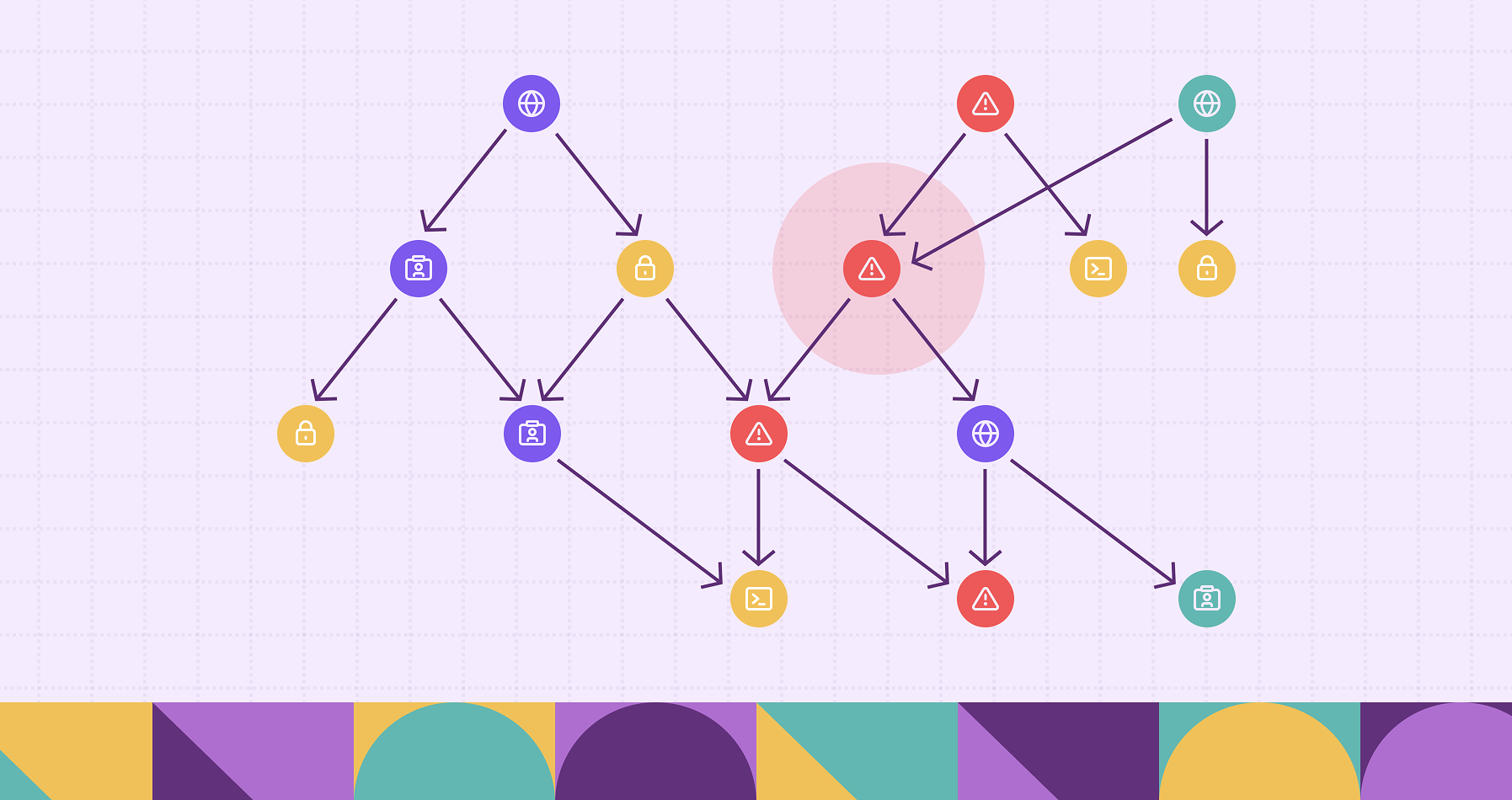
Figure: PuppyGraph Supported Data Sources

Advantages of PuppyGraph

Zero ETL: PuppyGraph lets you perform graph-based anomaly detection instantly, no ETL pipelines required. By directly connecting to your existing data warehouses and lakes, PuppyGraph eliminates the need for slow, failure-prone data transfers typical of traditional graph systems. You can detect anomalies and explore their relationships directly on live data, no preprocessing, no synchronization delay.
Petabyte-Level Scalability: PuppyGraph eliminates the scalability bottlenecks common in graph analytics by decoupling computation from storage. Through predicate pushdown, min/max pruning, and vectorized execution, it minimizes data scans while accelerating complex anomaly queries. Its auto-sharded, distributed architecture ensures consistent performance even across billions of nodes and edges.
Complex Queries in Seconds: Whether you’re searching for long transaction chains, structural outliers, or bridge nodes connecting separate communities, PuppyGraph executes even multi-hop and motif-based anomaly detection queries in seconds. Its distributed engine maximizes parallel execution for unmatched query speed, scaling performance simply by adding compute nodes.
Deploy to Detect in 10 Minutes: PuppyGraph’s lightweight deployment and zero-migration design let you start running anomaly detection queries in under 10 minutes. It works as a drop-in graph layer over existing systems, or even as a drop-in replacement for Neo4j, connecting seamlessly to your data and analytics tools with no code or data changes required.

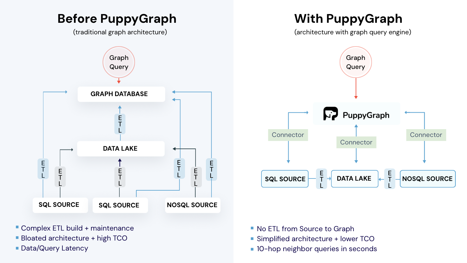
Figure: Architecture with Graph Database vs. with PuppyGraph

PuppyGraph supports both Gremlin and openCypher, making it simple to express anomaly detection rules as queries. For example, you can find nodes with unusually high degrees, detect edges forming unexpected triangles, or identify entities bridging disconnected clusters, all in a few lines of Cypher or Gremlin.

Such graph-based rules are intuitive and powerful, yet difficult to express in SQL. PuppyGraph turns them into real-time queries over production data, enabling analysts to detect, explain, and trace anomalies interactively.

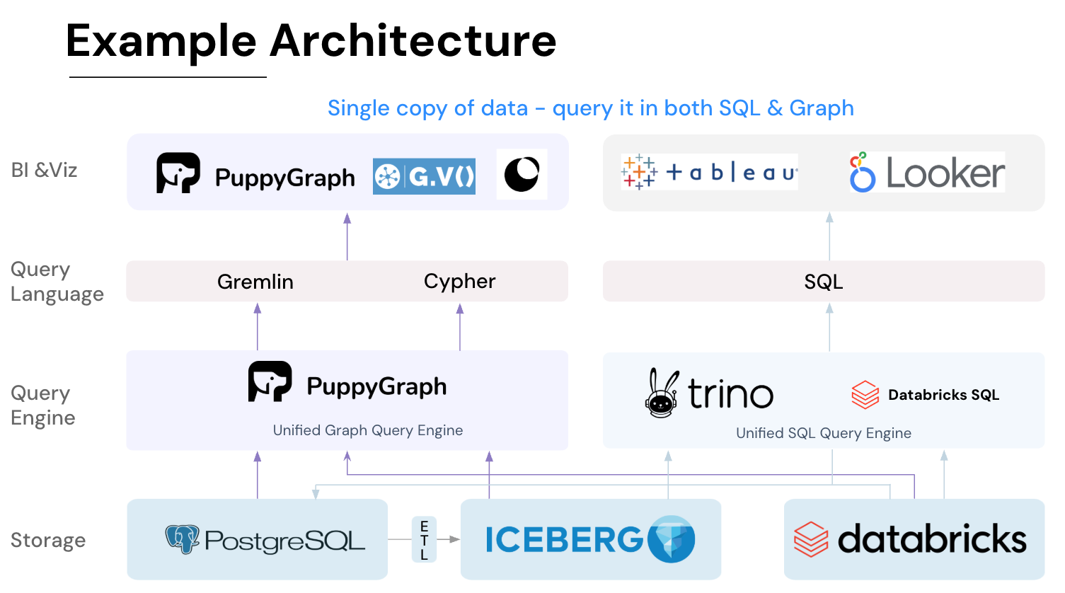
Figure: Example Architecture with PuppyGraph

As data ecosystems grow more complex, anomalies increasingly arise not in single records but in how entities connect and interact. PuppyGraph brings those patterns into focus, whether you’re detecting fraud rings, insider access paths, cybersecurity breaches, or knowledge inconsistencies in GraphRAG pipelines.

By allowing live query-driven anomaly exploration, PuppyGraph helps teams move seamlessly from detection to explanation, seeing not only what is anomalous, but why it emerged in the graph structure.

Most teams can get started by running PuppyGraph via Docker, AWS AMI, or GCP Marketplace, or deploy it securely inside their own VPC for full control. It’s the practical path from graph anomaly theory to real-time, query-driven anomaly detection, directly on your production data, at any scale.

Conclusion

Graph anomaly detection is a crucial capability for modern systems where relations matter. Rule-based and statistical methods like OddBall provide fast, interpretable, and often highly effective first-pass detection by exploiting simple egonet laws. Graph Neural Network approaches, such as Graph Autoencoders, learn expressive embeddings and can detect subtle structural–attribute interactions beyond heuristics.In production, hybrid pipelines (rule-based or statistic filters + deeper GNN refinement) combine the strengths of all approaches: speed, explainability, and adaptability.

Practical takeaways:

Start with simple rule-based or structural checks (degree limits, transaction frequency, egonet edges) to sanity-check data.
Use OddBall-like egonet residuals for quick interpretable alerts.
Add GNN-based reconstruction when you need to capture complex, multi-hop patterns or attribute interplay.
Always evaluate with precision@k, inspect top anomalies manually, and design pipelines that accommodate human feedback and evolving graph behavior.

If you’re ready to move from theory to practice, PuppyGraph lets you turn your existing data into a live graph for anomaly detection, instantly, without ETL or migration. Identify unusual nodes, edges, and subgraphs in real time, explore their neighborhoods, trace abnormal patterns, and uncover hidden risks across your relational data stack. Download the forever free PuppyGraph Developer Edition, or book a demo with our engineering team to see anomaly detection in action.

No items found.

Hao Wu

Software Engineer

Hao Wu is a Software Engineer with a strong foundation in computer science and algorithms. He earned his Bachelor’s degree in Computer Science from Fudan University and a Master’s degree from George Washington University, where he focused on graph databases.

See PuppyGraph

In Action

See PuppyGraph

In Action

Graph Your Data In 10 Minutes.

Get started with PuppyGraph!

PuppyGraph empowers you to seamlessly query one or multiple data stores as a unified graph model.