Building a Neural Network From Scratch — Just Numpy
In this article, I build a simple two-layer neural network from scratch and train it on the MNIST digit recognition dataset. Rather than relying on high-level frameworks, the focus is on understanding what actually happens inside a neural network, from forward propagation to backpropagation and parameter updates.
The problem that well be tackling is simple digit classification using the famous MNIST dataset. It classifies the handwriting digits and recognizes whats written.
The Math
Before diving into the code, it’s important to understand what we are actually building.
Each MNIST image has a resolution of 28×28 pixels, which means every image can be flattened into a vector of 784 pix...
Building a Neural Network From Scratch — Just Numpy
In this article, I build a simple two-layer neural network from scratch and train it on the MNIST digit recognition dataset. Rather than relying on high-level frameworks, the focus is on understanding what actually happens inside a neural network, from forward propagation to backpropagation and parameter updates.
The problem that well be tackling is simple digit classification using the famous MNIST dataset. It classifies the handwriting digits and recognizes whats written.
The Math
Before diving into the code, it’s important to understand what we are actually building.
Each MNIST image has a resolution of 28×28 pixels, which means every image can be flattened into a vector of 784 pixel values. If we have m training images, we can stack these vectors together to form a matrix X. Initially, this gives us a matrix of shape (m × 784), where each row corresponds to one training example. However, for efficient vectorized computation in neural networks, we transpose this matrix so that X has shape (784 × m), meaning each column now represents a single image. This layout allows us to process all training examples simultaneously using matrix multiplication during forward and backward propagation.

Nueral Network
Now that the input data is properly represented as a matrix, we can define the structure of our neural network.
- The input layer consists of 784 units, one for each pixel in the flattened 28×28 image. These values are fed directly into the network as the input vector for each sample.
- The hidden layer contains 10 neurons. Each neuron in this layer is fully connected to all 784 input pixels, meaning it learns a weighted combination of the entire image. After computing this weighted sum and adding a bias term, we apply a non-linear activation function (ReLU). This non-linearity is crucial, as it allows the network to learn complex patterns rather than being limited to simple linear relationships. Intuitively, the hidden layer begins to act as a feature extractor, learning to respond to meaningful patterns in the image such as strokes, edges, or curves that are useful for distinguishing digits.
- The output layer also consists of 10 neurons, one for each possible digit class from 0 to 9. Each output neuron receives input from all neurons in the hidden layer and produces a raw score representing how strongly the network believes the input image belongs to that class.

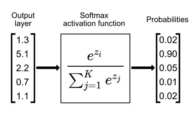
These raw scores are then passed through a softmax function, which converts them into probabilities. The softmax ensures that all output values lie between 0 and 1 and that they sum to 1, allowing the network’s prediction to be interpreted as a probability distribution over the ten digit classes.
At inference time, the digit with the highest probability is selected as the network’s final prediction. During training, these predicted probabilities are compared against the true labels, and the error is propagated backward through the network to update the weights and biases.

Forward Propagation
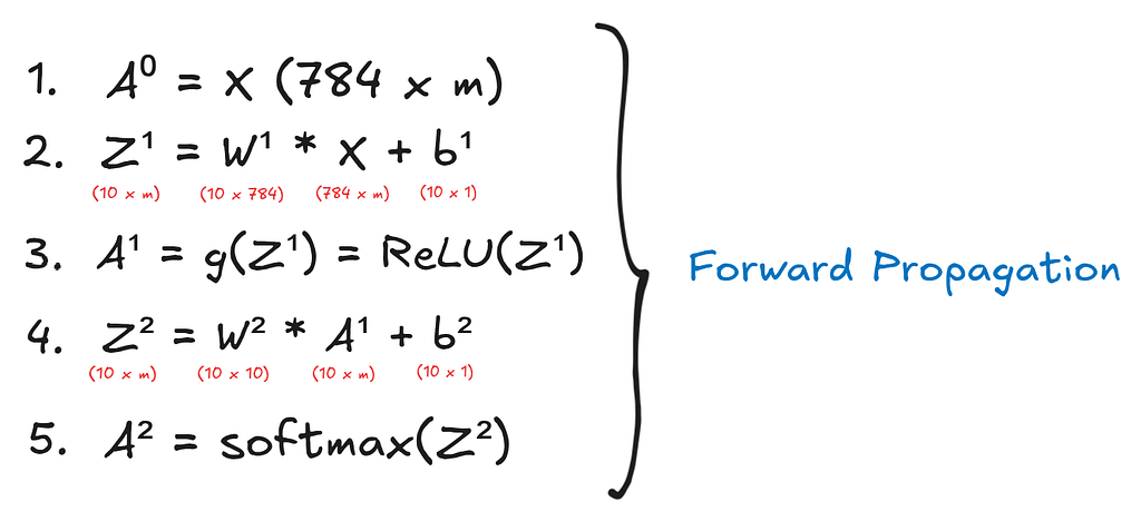
Forward propagation is the process by which the neural network takes an input image and produces a prediction.
We begin by computing
- Z[1] = W[1]X + b[1] — This first step forms a weighted sum of the input pixels for each hidden neuron. Each neuron looks at all 784 pixels, multiplies them by learned weights, and adds a bias. This allows the network to measure how strongly certain patterns appear in the image.
- A[1] = ReLU(Z[1]) — Then, ReLU keeps positive values and sets negative values to zero. This introduces non-linearity, allowing the network to learn complex patterns instead of behaving like a simple linear model.
- Z[2] = W[2]A[1] + b[2] — Here, the features learned by the hidden layer are combined to produce a score for each digit class.
- A[2] = softmax(Z[2]) — Finally softmax converts these scores into probabilities that sum to one, making the network’s output easy to interpret. The digit with the highest probability is chosen as the final prediction.
def ReLU(Z): return np.maximum(Z, 0) def softmax(Z): return np.exp(Z) / sum(np.exp(Z)) def forward_prop(W1, b1, W2, b2, X): Z1 = W1.dot(X) + b1 A1 = ReLU(Z1) Z2 = W2.dot(A1) + b2 A2 = softmax(Z2) return Z1, A1, Z2, A2
Backward Propagation
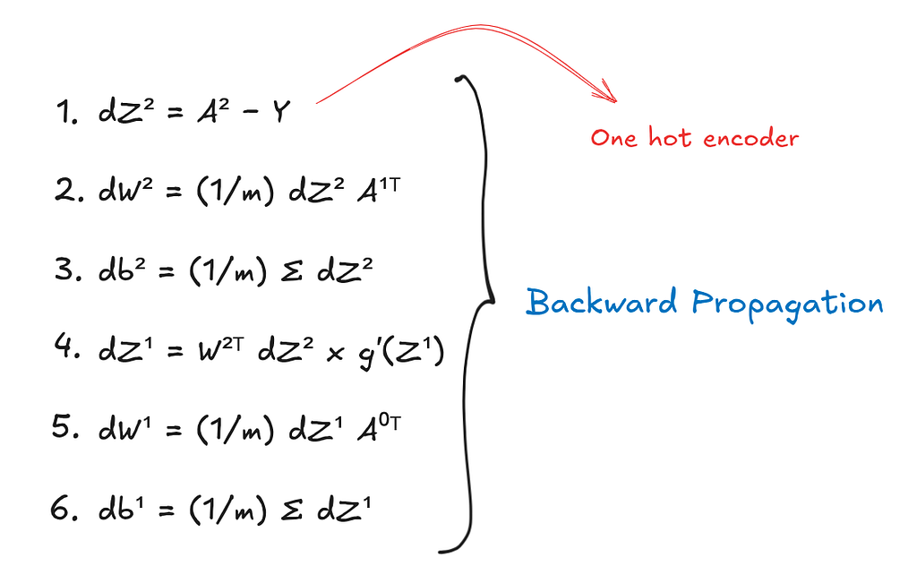
Backward propagation is how the network learns from its mistakes. After forward propagation produces a prediction, we compare it with the true label and propagate the error backward through the network to determine how each parameter should be adjusted.
- dZ[2] = A[2] − Y — This term represents the error in the output layer. Since we use a softmax activation combined with cross-entropy loss, the gradient simplifies neatly to the difference between the predicted probabilities and the true labels. This tells us how much each output neuron overestimated or underestimated its prediction.
- dW[2] = (1/m) dZ[2] A[1]ᵀ — Each weight in the output layer connects a hidden neuron to an output neuron. This formula measures how much each hidden neuron contributed to the output error, averaged over all training examples. Intuitively, if a hidden neuron was highly active and led to a large error, the corresponding weight should be updated more strongly.
- dB[2] = (1/m) Σ dZ[2] — Biases affect all inputs equally, so their gradients are simply the average error across the batch.
- dZ[1] = W[2]ᵀ dZ[2] * g′(Z[1]) — Here, the transpose of W[2] redistributes the output error to the hidden neurons based on how strongly they influenced the output. This error is then multiplied element-wise by the derivative of the ReLU activation. This step ensures that only neurons that were active during the forward pass receive gradient updates (its basically like deactivating the activation function).
- dW[1] = (1/m) dZ[1] A[0]ᵀ — This formula measures how much each input pixel contributed to the error in the hidden layer. It allows the network to learn which pixel patterns were responsible for incorrect predictions.
- dB[1] = (1/m) Σ dZ[1] — As with the output layer, this captures the average error associated with each hidden neuron.
def ReLU_deriv(Z): return Z > 0 def one_hot(Y): one_hot_Y = np.zeros((Y.size, Y.max() + 1)) one_hot_Y[np.arange(Y.size), Y] = 1 one_hot_Y = one_hot_Y.T return one_hot_Y def backward_prop(Z1, A1, Z2, A2, W1, W2, X, Y): one_hot_Y = one_hot(Y) dZ2 = A2 - one_hot_Y dW2 = 1 / m * dZ2.dot(A1.T) db2 = 1 / m * np.sum(dZ2) dZ1 = W2.T.dot(dZ2) * ReLU_deriv(Z1) dW1 = 1 / m * dZ1.dot(X.T) db1 = 1 / m * np.sum(dZ1) return dW1, db1, dW2, db2
Together, these gradients tell us exactly how each weight and bias should be adjusted to reduce the loss. Backpropagation is essentially an efficient application of the chain rule that assigns responsibility for the prediction error across all layers of the network.
Parameter Updates
After computing the gradients during backpropagation, the final step is to update the network’s parameters so that it performs better on the next forward pass. This is done using gradient descent, an optimization method that adjusts parameters in the direction that reduces the loss.
- W[2] = W[2] − α dW[2] — Here, dW[2] tells us how changing each weight would affect the loss. The learning rate α controls how large a step we take in the opposite direction of the gradient. Subtracting the gradient ensures that the weights move toward values that reduce the prediction error.
- b[2] = b[2] − α db[2] — Biases shift the output of neurons independently of the input, and updating them allows the network to correct systematic overconfidence or underconfidence in certain classes.
- W[1] = W[1] − α dW[1] — updates the connections between the input pixels and hidden neurons, strengthening connections that helped correct predictions and weakening those that contributed to errors.
- b[1] = b[1] − α db[1] — adjusts how easily each hidden neuron activates.
def update_params(W1, b1, W2, b2, dW1, db1, dW2, db2, alpha): W1 = W1 - alpha * dW1 b1 = b1 - alpha * db1 W2 = W2 - alpha * dW2 b2 = b2 - alpha * db2 return W1, b1, W2, b2
Together, these updates slightly modify the network’s behaviour after each training step. Repeating this process over many iterations gradually reduces the loss, allowing the network to learn meaningful features and improve its predictions.

This process repeats itself until the we get acceptable results.
def get_predictions(A2): return np.argmax(A2, 0) def get_accuracy(predictions, Y): print(predictions, Y) return np.sum(predictions == Y) / Y.size def gradient_descent(X, Y, alpha, iterations): W1, b1, W2, b2 = init_params() for i in range(iterations): Z1, A1, Z2, A2 = forward_prop(W1, b1, W2, b2, X) dW1, db1, dW2, db2 = backward_prop(Z1, A1, Z2, A2, W1, W2, X, Y) W1, b1, W2, b2 = update_params(W1, b1, W2, b2, dW1, db1, dW2, db2, alpha) if i % 10 == 0: print("Iteration: ", i) predictions = get_predictions(A2) print("Accuracy: ", get_accuracy(predictions, Y)) return W1, b1, W2, b2

You can find the code for the network here.
With an accuracy of around 85%, this model can definitely be improved by introducing more layers or playing around with the activation functions and hyperparameters. However the goal of this article is to provide a basic understanding without worrying too much about the performance. Credit to Samson Zhang for his video on the topic.
Building a Neural Network from scratch — Just numpy was originally published in Towards AI on Medium, where people are continuing the conversation by highlighting and responding to this story.