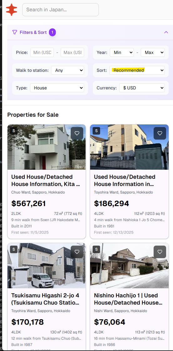
I turned property listings into vectors for Nippon Homes and used them to surface homes you’re likely to view.. Currently, NipponHomes has around 150k active listings at any given time and 8k monthly users.

---

The Core Idea: Properties as Vectors

Every property is a point in 9-dimensional space. Similar properties cluster together—small Tokyo condos in one region, spacious countryside houses in another.

When you browse listings, we’re essentially watching which regions of this space you’re drawn to. After a few views, we can compute your "preference center" and find other properties nearby.

Mathematically, we represent each listing as a 9d feature vector:

v⃗listing=[d0,d1,d2,…,d8]∈R9\vec{v}_{\text{listing}} = [d_0, d_1, d_2, \ldots, d_8] \in \mathbb{R}^9

Each dimension captures something meaningful about the property.

Seeing It In Action

Here are 6 Tokyo condos and 6 Hokkaido houses from the database, all similarly priced (¥22M-¥40M). Despite similar prices, they live in completely different regions of our 9-dimensional space.

Since we can’t visualize 9 dimensions, I’ve used Principal Component Analysis (PCA) to project them into 3D:

Loading 3D visualization...

Notice the clear separation: blue points (Tokyo condos) cluster together in one region, while orange points (Hokkaido houses) form their own distinct group. This happens because Tokyo condos are smaller (48-64㎡) with higher price-per-㎡, while Hokkaido houses are spacious (74-251㎡) with more rooms.

When you browse Tokyo condos, your preference vector moves toward the blue cluster. The system then finds other nearby blue points (similar condos) you haven’t seen yet.

---

The 9 Dimensions We Track

Here’s the actual PostgreSQL trigger function called get_personalized_rankings that computes the feature vector whenever a listing is inserted or updated:

DECLARE
vector_data vector(9);
normalized_rooms TEXT;
room_count INTEGER;
BEGIN
normalized_rooms := normalize_rooms(NEW.rooms);
room_count := COALESCE(
(regexp_match(normalized_rooms, '(\d+)'))[1]::integer,
3
);

-- Scaling strategy: heuristic z-score normalization
-- Centers ≈ dataset mean (e.g., 100m² actual mean: 100.7m²)
-- Scales ≈ "practical range" (~0.5-1σ), NOT true standard deviations
-- This keeps most values in [-2, +2] and prevents high-variance
-- features from dominating distance calculations.
-- Binary features use ±1 for equal "vote weight" regardless of
-- class imbalance.

vector_data := ARRAY[
-- Dim 0: Size — center 100m² ≈ mean, scale 50 (~0.6σ, actual σ≈85)
(COALESCE(NEW.size_sqm, 100) - 100.0) / 50.0,

-- Dim 1: Price — log-scaled, center 17 ≈ ln(¥24M) ≈ actual mean 17.03
(LN(GREATEST(COALESCE(NEW.price, 25000000), 1000000)) - 17.0) / 1.0,

-- Dim 2: Price/m² — center 300k (actual mean ~454k, Tokyo skews high)
-- Scale 200k (~0.3σ) compresses outliers intentionally
CASE
WHEN COALESCE(NEW.size_sqm, 0) > 10
THEN (COALESCE(NEW.price, 0) / NEW.size_sqm - 300000.0) / 200000.0
ELSE 0
END,

-- Dim 3: Age — center 25 years, scale 15
(EXTRACT(YEAR FROM CURRENT_DATE) - COALESCE(NEW.year_built, 1995) - 25.0) / 15.0,

-- Dim 4: Room count — center 3.5, scale 1.5
(room_count - 3.5) / 1.5,

-- Dim 5-8: Binary features use ±1 (not normalized to class imbalance)
-- This gives equal weight in distance calculations

-- Dim 5: LDK flag (modern layout)
CASE WHEN normalized_rooms LIKE '%LDK%' THEN 1.0 ELSE -1.0 END,

-- Dim 6: Listing type (house vs condo)
CASE WHEN NEW.listing_type = '中古一戸建て' THEN 1.0 ELSE -1.0 END,

-- Dim 7: Size efficiency (sqm per room) — center 25, scale 10
(COALESCE(NEW.size_sqm, 100) / GREATEST(room_count, 1) - 25.0) / 10.0,

-- Dim 8: Has storage room (+S or SLDK pattern)
CASE WHEN normalized_rooms ~ '\+S|S[LDK]' THEN 1.0 ELSE -1.0 END

]::vector(9);

INSERT INTO vecs.listing_vecs (id, vec, listing_id)
VALUES (NEW.id, vector_data, NEW.listing_id)
ON CONFLICT (id)
DO UPDATE SET
vec = EXCLUDED.vec,
listing_id = EXCLUDED.listing_id;

RETURN NEW;
END;

The scaling isn’t mathematically pure z-score normalization, but it works well for similarity search. The key insight: using ~0.5-1σ as the scale (instead of true σ) keeps most values bounded and prevents high-variance features from dominating.

---

Computing Your Preference Vector

As you browse, we track which listings you view. After you’ve seen at least 3 properties, we compute your preference centroid—the average of all vectors you’ve engaged with.

Generic formula for n vectors:

p⃗user=1n∑i=1nv⃗i\vec{p}_{\text{user}} = \frac{1}{n} \sum_{i=1}^{n} \vec{v}_i

Example: If you viewed three properties:

• A small Tokyo condo: v⃗1=[−1,0.5,1,−0.5,−1,1,−1,−0.5,−1]\vec{v}_1 = [-1, 0.5, 1, -0.5, -1, 1, -1, -0.5, -1]
• Another small condo: v⃗2=[−0.8,0.3,0.8,0,−0.7,1,−1,−0.3,−1]\vec{v}_2 = [-0.8, 0.3, 0.8, 0, -0.7, 1, -1, -0.3, -1]
• A compact apartment: v⃗3=[−1.2,0.4,1.2,−0.3,−1,1,−1,−0.7,1]\vec{v}_3 = [-1.2, 0.4, 1.2, -0.3, -1, 1, -1, -0.7, 1]

Computing the centroid with 3 vectors:

p⃗user=13(v⃗1+v⃗2+v⃗3)\vec{p}_{\text{user}} = \frac{1}{3}(\vec{v}_1 + \vec{v}_2 + \vec{v}_3) p⃗user=[−1.0,0.4,1.0,−0.27,−0.9,1.0,−1.0,−0.5,−0.33]\vec{p}_{\text{user}} = [-1.0, 0.4, 1.0, -0.27, -0.9, 1.0, -1.0, -0.5, -0.33]

This centroid vector represents your inferred preference profile. Here’s how it looks in 3D space:

Loading preference centroid visualization...

---

Finding Similar Properties

With your preference vector computed, we find the closest unviewed properties using Euclidean distance (L2):

distance(p⃗,v⃗)=∑i=08(pi−vi)2\text{distance}(\vec{p}, \vec{v}) = \sqrt{\sum_{i=0}^{8} (p_i - v_i)^2}

To convert distance into a similarity score between 0 and 1, we use:

similarity=11+distance\text{similarity} = \frac{1}{1 + \text{distance}}

This formula has nice properties:

• Distance = 0 → Similarity = 1 (perfect match)
• Distance = 1 → Similarity = 0.5
• Distance → ∞ → Similarity → 0

---

Making It Fast: HNSW Indexing

With thousands of listings, computing distances to every property would be slow. We use HNSW (Hierarchical Navigable Small World) indexing via pgvector:

CREATE INDEX listing_vecs_vec_idx
ON vecs.listing_vecs
USING hnsw (vec vector_l2_ops);

HNSW builds a graph structure that allows approximate nearest-neighbor search in O(log n) time instead of O(n). For our ~50k listings, this means queries complete in milliseconds.

---

The Complete Query

Here’s the actual PostgreSQL function that powers recommendations:

WITH preference_vector AS (
-- Compute centroid of viewed listings
SELECT AVG(v.vec)::vector(9) as pref_vec
FROM vecs.listing_vecs v
WHERE v.listing_id = ANY(viewed_ids)
),
top_matches AS (
SELECT
lv.listing_id,
-- Convert distance to similarity score
(1.0 / (1.0 + (lv.vec <-> pv.pref_vec))) as score
FROM vecs.listing_vecs lv
CROSS JOIN preference_vector pv
WHERE
pv.pref_vec IS NOT NULL
AND lv.listing_id != ALL(viewed_ids)  -- Exclude already viewed
ORDER BY lv.vec <-> pv.pref_vec  -- L2 distance operator
LIMIT 100
)
SELECT * FROM top_matches ORDER BY score DESC;

The <-> operator computes L2 distance and leverages the HNSW index automatically.

---

Exploration vs. Exploitation (adding diversity to ranked results)

A pure similarity-based system has a problem: it can create filter bubbles. If you only see properties similar to what you’ve viewed, you might miss great options outside your initial exploration. Inside the Next.JS function, after we call get_personalization_rankings to re-rank the listings, we then sort them in a format such that we interleave non-matches, to give the user a chance to explore non-similar listings (to add diversity).

We address this with interleaving:

results=[relevant0,random0,relevant1,random1,…]\text{results} = [\text{relevant}_0, \text{random}_0, \text{relevant}_1, \text{random}_1, \ldots]

Every other result is a random property from the candidate set. This ensures:

1. You see your best matches
2. You discover properties you might not have found otherwise
3. The system learns from your reactions to diverse options

---

What’s Next?

This is version 1. Future improvements that I have pondered about:

• Dwell-time weighting: Properties you spent more time viewing should influence your preference vector more. Tried to implement this but ran into some errors. May revisit.

• Recency decay: Recently viewed listings matter more than listing views from last week.

• Learning to rank (LTR): Meta, Google, and other big companies use LTR to rank their ads effectively. From the developers that I spoke to there, it sounded like they tend to just use XGBoost for their late stage rankers. There’s a few things I want to experiment in this area:

• LightGBM/XGBoost with LambdaMART

• Vowpal Wabbit for multi-armed bandits (Use click-through data to tune dimension weights)

• Simple MLP neural net

• Image embeddings: I’ve prototyped this for Hokkaido listings using LiquidAI’s LFM2-VL-1.6B model. Visual embeddings from property photos are fused with the 9-dimensional metadata through an MLP into 128-dimensional vectors for similarity search. I’m kinda GPU-poor though so, I’ll stick to the basics for now.

For now, the simple centroid approach works remarkably well. Sometimes the best solution is the simplest one.

---

Built with PostgreSQL, pgvector, and a healthy appreciation for linear algebra.