2026 will be the year of real-time video generation

Video diffusion models are incredibly popular. They have come a long way from Will Smith shovelling spaghetti into his face back in 2023! The recent release of Sora2, for example, has led to an explosion of AI generated video (my favourite of which has been the doorbell camera videos of cats, shown below).

While there can be no doubt that video is crossing the uncanny valley and becoming very close to perfectly real, there are still some limitations. One of these is the fact that a video has to be generated all at once before it can be shown to the user. This is perfectly fine in most use cases, but for my personal field of work, its an issue. When working with conversational Avatars, we want realtime, streaming video generation. What do I mean by this?

We need frames of video to appear in a continuous manor, causally (e.g. only using information available in the past), and with a small enough delay (usually <200ms).

Typical video diffusion models work on a fixed sized chunk of frames, and generate all at the same time. This is a relatively straightforward setting which makes training easier, but has several drawbacks. The most obvious issue being that the length of any generated videos has to be the same as the length at training. It is not possible to continue the generation for infinite length videos. Also the use of self-attention means that all frames attend to all others. Even though engineering feats such as flash-linear-attention make this less of a burden, it is still a significant slow down. So whats the alternative?

Autoregressive Diffusion Models

The way to create infinite length videos is to train an autoregressive model. These models take some history in the form of past frames and use this to generate some future frames. At training, we can use ground truth video, with some frames as the past and predict the future frames for which we have ground truth. Then, for inference, we can generate some frames, make them the past, generate more and repeat ad-infinitum (as in the above diagram). Seems easy right? Let’s try it…

Note: For all experiments here, I am finetuning Wan2.1–1.3B with a LoRA of rank 128 and alpha=64 on a dataset of ~100k videos. This is not the best possible setting and is far behind SOTA.

… and it doesn’t look great. What’s going on here? The key issue is the mismatch between training and inference. At training the model always gets perfect ground truth as the past input. It learns to mimic this very closely. However, it is not perfect and will produce some small errors. These are then passed as the history at inference, and the model will use imperfect history treating it as ground truth. In this way, errors quickly compound leading to unstable generations, we call this error accumulation. This method of training on the ground truth is called teacher forcing and its something we want to avoid.

This is a known problem in other models, going back at least as far as RNNs. The solution in that case is obvious, we perform what is called a ‘rollout’ applying the forward process a few times so that the model is trained with its own outputs as history. However, for video diffusion this is not so simple. The main reason being that a diffusion model requires anything from a few dozen to a few hundred denoising steps (which are very computationally expensive for video models) per inference step. So to do one training step with 3 rollouts and a modest 50 denoising steps, you would need to do 150 forward passes per inference step. This is both impractical, the training time would be enormous, and also can lead to gradient issues. What are the alternatives?

Diffusion Forcing

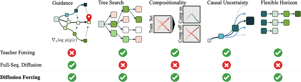
One of the first works to address the issue of error accumulation in teacher-forcing models is diffusion forcing. The key idea here is that we can use noise as masking. You can view this as noise as uncertainty. This lets us treat fully noisy samples as masked (fully uncertain). To do this, the change is fairly straightforward. Instead of treating a sequence of length L as a single step in the diffusion process with a corresponding timestep t, we treat each frame independently, assigning each its own timestep. For training this is a simple modification, we just apply the noise to each frame indepedently. However, at inference, diffusion forcing opens up a host of tricks.

• Autoregressive generation: Even though the model is not trained auto-regressively, it can be used in this way at inference. By applying noise only to the future frames, leaving the past without noise, it is able to perform rollouts. We’re effectively saying, the past is known, the future is uncertain, predict the future frames.
• Error Correction: By leaving past frames with a very low noise level, the model knows to treat these as slightly corrupted, and therefore learns to correct its own errors. This prevents error accumulation! We say, there is some uncertainty in the past, knowing this, predict the future.
• Future Uncertainty Modelling: The model is able to make predictions about the future even without any potential conditions by performing just a few denoising steps, and leaving the uncertainty in the form of nosie. We are saying, make prior predictions about the future, without any evidence, but leave uncertainty.

Ok so this helps a lot with allowing for streaming! However, what it doesn’t do is improve the speed of the models. They will still be a long way from realtime. To understand the methods that get us to realtime, we need to first understand model distillation.

Model Distillation

Model distillation is an old and well-known trick that enables the training of a student model from a teacher. In the case of typical model distillation, it is quite a surprise that the student model performs better when distilled from a teacher when compared with the same student trained on the teacher model’s dataset. Diffusion training relies on synthetic supervision, predicting noise or flow from noisy inputs, where the optimal target is implicitly defined by the data distribution. Distillation replaces this noisy, high-variance supervision with targets produced by a trained teacher, providing smoother, lower-entropy pseudo-labels that better reflect the learned score field. You can think of this as the teacher giving the student explict guidance on what it needs predict, rather than learning it from the data distribution. This makes the task much easier and allows for significant benefits:

• Step Distillation: A powerful pretrained teacher can be distilled into a model that works in just one (or a few) steps, drastically reducing inference time.
• Architecture Distillation: A model with more parameters can be distilled into a model with fewer. This also speeds up inference.
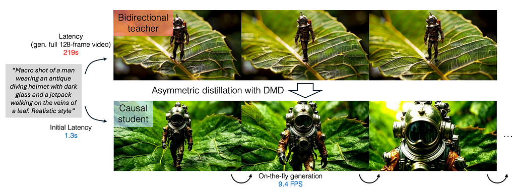
• Causality Distillation: We can distill bidirectional teacher model into a student model that is causal (cannot ‘see’ the future frames). This is obviously useful in autoregressive models where the future is not available, but also reduces the number of attention calculations.

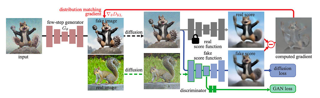
In practise, the student is not distilled using the teacher models inputs and outputs, but instead the score functions of the teacher are used to inform the student. The score function is the gradient of log probability density with respect to the data. In simpler terms, it shows what changes can be make to an input to move it closer to pure data and away from noise. This is clearly a useful signal to the student, and is exploited by several papers that I would love to detail in the future.

CausVid

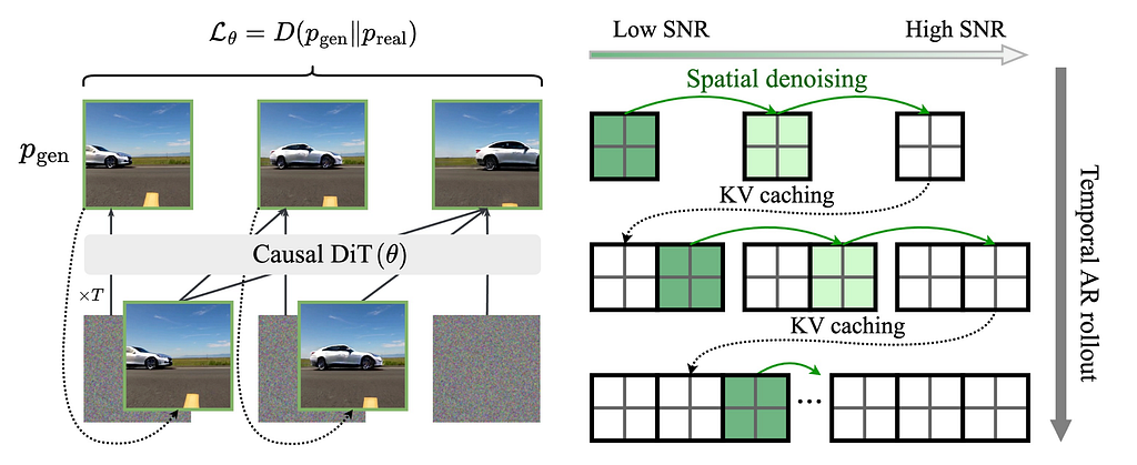
A few works look to tackle the issue of realtime auto-regressive video diffusion models with this new tool of distillation under the belt. One of these is CausVid, there are a few innovations here. The first is the design of a block-causal attention mechanism that allows each token to attend to all others in the same and previous blocks, but not the future. It then uses DMD to distill a bidirectional model that requires 50 denoising steps, into this block-causal model that needs only 4. The student model uses diffusion forcing. They also improve convergence by directly using ODE trajectories, using the noise as input and the denoising steps from the teacher as the target.

With this autoregressive model, it is also possible to do KV caching, which allows the model to run a ~10fps on a single GPU with infinite length and good results! But we’re still a bit off realtime.

Self-Forcing

Self forcing finally lets us do what we wanted to do with rollouts, thanks to distillation. By using a few step model distilled from a more powerful one, it is far more practical to perform rollout. This means we can train the model to correct its own mistakes directly, rather than simply marking frames as uncertain (as in diffusion forcing). While the use of a distilled model makes it possible to perform to run training in a reasonable time, there is still an issue with the gradient computation. To overcome this only one denoising step per frame uses a gradient computation, while the others are forward passes only, the algorithm works (roughly) as follows in pytorch-ish psuedocode:

def train_step(model, noise, n_denoise_steps=4): history = [] for frame in frame: noise_frame = noise[frame] step_for_grad = random(n_denoise_steps) for t in range(n_denoise_steps): if t == step_for_grad: noise_frame = diffusion_step(noise_frame, model, t) compute_gradients() else: with no_grad(): noise_frame = diffusion_step(noise_frame, model, t) update_model_parameters()

In addition, the self-forcing paper also simulates the KV-caching process during the training rollout. This matches what happens at inference and further improves the inference quality. The result is even faster generations (16FPS)! However, this does stop working after long generation due to a mismatch in the RoPE mechanism.

There are works that address this, for example Infinity RoPE, which addresses the issues by making the positional embeddings relative to the current frame index, and storing a sink frame plus the last frame only in the KV cache. This stops the deterioration.

Avatar Specific Models

The above are really excellent models for general video generation, but there is some additional work that needs to be done for Avatars. Two recent works come to mind that use some or all of the above concepts.

LiveAvatar

LiveAvatar is a work from Alibaba which pretrains the WanS2V model (a 16B DiT) using diffusion forcing on the AVSpeech dataset with a block-wise causal mask (like CausVid). They then perform self forcing distillation to distill to 4 steps. They also use a relative (rolling) RoPE and an attention sink in the form of a reference frame which always remains ahead of the target frame.

By staggering the diffusion steps, they are able to have a separate GPU do each step, with batching. With a 4 step model, a total of 5H100s are needed (one for VAE decoding), which is a big limitation. However, it is able to run at 20fps.

Talking Machines

Talking machines is another great work from Character AI that also builds on the work outlined above. It starts with the Wan2.1 14B model, first finetuning it to work at 512x512 resolution, then adding an audio cross attention layer to do the lip sync. This gives a teacher model, which they distil into an autoregressive student, similar to CausVid, except instead of using a diffusion forcing training setup, they train the student with a fixed timestep shared across frames. They also slightly change up the masking, so that a reference frame is always seen by all latents.

Conclusions

Video diffusion is quickly becoming quick! It’s looking increasingly likely that we will be able to reach near-state of the art quality with models that can be run continuously, in realtime and for minimal cost. This will open up a whole host of applications, particularly in the Avatar space. Although, it will yet again raise the question of what we can trust online.

I believe that these models will become even faster through several methods. In particular, while there has been a lot of work on step and causality distillation, there is more that could be done with distilling to smaller architectures. I also think LoRA like adaptations per-person or per-population (e.g. photoreal vs cartoon) could enable this, by reducing the amount of knowledge needed in a model and enabling smaller and therefore faster architectures.

These models are extremely powerful, and we are likely only a few breakthroughs away from Sora2 quality in realtime. 2026 will be an exciting year!

Towards Streaming Video Diffusion was originally published in Towards AI on Medium, where people are continuing the conversation by highlighting and responding to this story.