• 23 Dec, 2025 *

Large Language Models are all the rage right now. It’s been a goal of mine to understand how these models work, so I’ve been ramping up on their academic lineage and implementing what I learn in code. For more background on these topics, I highly recommend Andrej Karpathy’s Zero to Hero series on YouTube.

This post is Part 1 of an n-part series on language modeling. Language modeling has a diverse range of problems within it, such as translation, semantic analysis, and prediction. For this series we will be looking at next token prediction. Specifically, given a sequence of tokens (like characters or words), we want to create a model which predicts the next token. Mathematically this amounts to finding a model which maximizes the likelihood of the next token conditioned on the previous tokens.

In this series, we are going to start from simple models and work our way up to the modern state of the art like transformers and also some more exotic architectures like text diffusion models.

Neural Probabilistic Language Model

Some of the first attempts of language prediction used frequency-based n-gram models. With n-gram models, the predictions are based on the frequency of n-grams in the training corpus. The work from Bengio et al. improved upon the existing state of the art n-gram models way back in 2003 with their “Neural Probabilistic Language Model”. They were one of the first to successfully apply neural networks to the language prediction task. The main contribution from this paper was a solution to the curse of dimensionality problem via learned embeddings.

To understand the curse of dimensionality, consider the following sentences:

The dog is running in the yard

The cat is drinking in the kitchen

The man is running in the street

If only the first two are in the training set, then a classical n-gram approach, where the probabilities are assigned based on the frequency of their occurrence in the training data, will fail to predict the last sentence as very likely, since it never appeared in training. This seems wrong, since all three sentences are grammatically and semantically similar.

The root cause of this is the set of possible sentences is an extremely high dimensional space (and hence is cursed :)), and the n-gram approach has no mechanism to transfer probability mass found during training to unseen sentences.

Overcoming the Curse of Dimensionality

Bengio found a way around this using learned word embeddings. Embeddings are real-valued vectors that are used to numerically represent words. The vectors encode the syntax and semantics of each word. What is neat about this encoding is that it allows us to perform arithmetic on words, and to measure mathematically how close they are to each other via the geometric interpretation of vectors. So words with similar meaning like “mammal”, “dog”, “human” will have similar vectors and words like “it”, “the”, “a”, “and” will have similar vectors, however those two groups of vectors would not be close to each other in the vector space.

As a simple example, we can suppose the embedding vector is three dimensional as seen below:

x→=[part of speechinanimatecolor]

Each word would have a vector of its own, for example mammal might be (3.6, -2.4, 0.1) and dog might be (3.7, -2.3, 0.5). We can then compute the Euclidean distance between them. Semantically similar words will have a distance near zero.

So you may be thinking, OK then we just have to somehow come up with the “most important” features of a word, like part of speech and its semantic usage and create vectors that encode these that we come up with. But Bengio found that we can let the model learn what “features” are important based on the statistics of the training data. We don’t have to explicitly say that the first element of each vector represents part of speech, the second whether it represents something inanimate, etc. The model learns these values for us via backpropagation.

The reason this technique overcomes the curse of dimensionality is that predicting the next word given a sequence of words is likely to pick any word with a vector which is similar to that seen in the training set, not just the word that was seen in the training set. So predicting the next word of

The man was hungry so he ate the ____.

would assign a high likelihood to any type of word that semantically describes food, even if the only instance of the phrase in training was e.g. “The man was hungry so he ate the banana”. This is what it means to “transfer” probability mass to similar words. This transfer allows for an exponential increase in the sequences which the model finds likely, leading to better generalization.

Visualizing Embeddings with t-SNE

Unfortunately, humans can’t visualize spaces with a high number of dimensions, given our senses have evolved in three dimensional space. This makes gaining intuition of high-dimensional objects like embedding vectors difficult.

Fortunately, there are algorithms such as t-SNE for projecting high-dimension vectors into two dimensions. This allows us some sense of the clustering that is present among the embedding vectors and gives us intuition for the similarity between the words.

You can see an example of this below that uses the TinyStories dataset. It uses t-SNE to project the 32-dimensional embeddings of lower case letters to two dimensions.

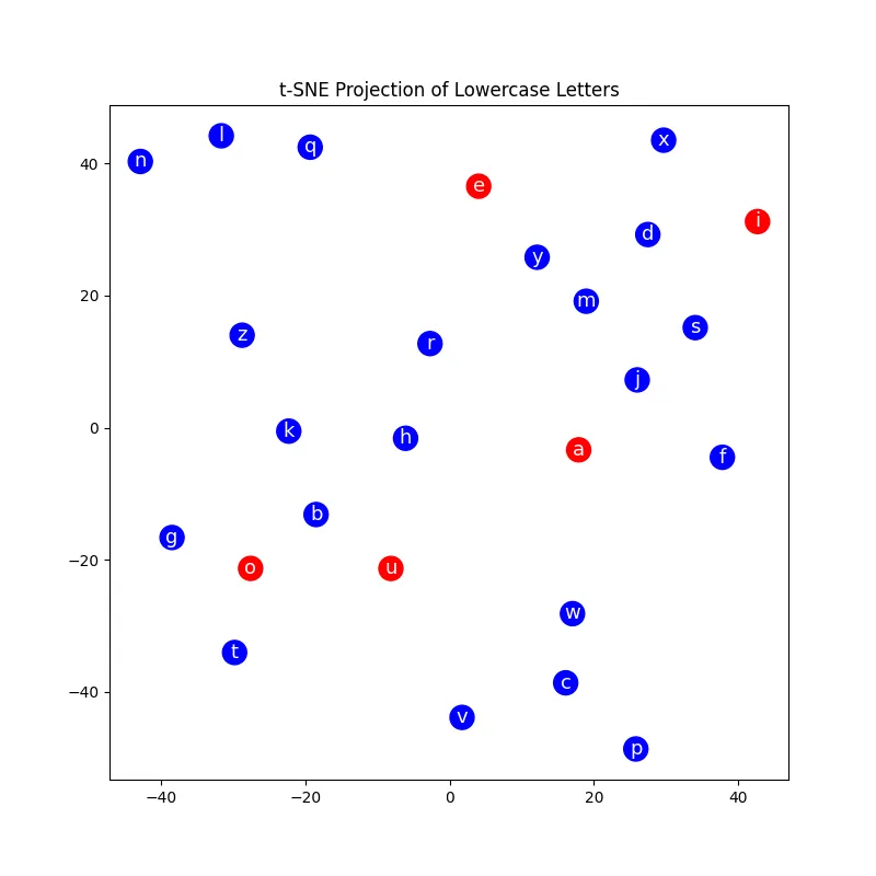
The vowels are in red and consonants in blue. The image above is the t-SNE projection from the random initialization of the embedding vector.

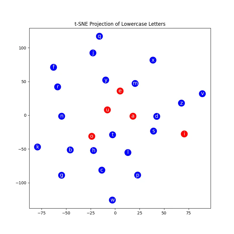
The image above is the projection after 30,000 training iterations of character-level language model that uses Bengio-style embeddings for each character. You can see as the training progresses, the embeddings of semantically similar characters like vowels begin to cluster together.

Building the Model

Let’s implement a model similar to the one from the Bengio paper. We will use the TinyStories dataset. This dataset features a collection of short stories generated from ChatGPT. We will train a character-level language model using PyTorch that will be able to generate new short stories for us. Note that below will just have snippets; here is a colab notebook if you want to have a complete picture.

Prepping the Dataset

The first step is to get familiar with the data. We need to download the dataset and convert it into a format that we can use for training:

import torch
import torch.nn.functional as F
import matplotlib.pyplot as plt
import numpy as np

from datasets import load_dataset

d = load_dataset('roneneldan/TinyStories')
data_trn = list(d['train'].to_pandas().to_dict().values())
data_val = list(d['validation'].to_pandas().to_dict().values())

# Get the unique characters across the training set
unique_chars = set()

for story_dict in data_trn:
for story_text in story_dict.values():
unique_chars.update(set(story_text))

unique_chars = ''.join(sorted(unique_chars))

# We use '^' as a special start character in the model
assert '^' not in unique_chars

I validated experimentally that ‘^’ isn’t in the training set at all, so I opted to use it as a special starting character as we will see later. Now we can create our char-to-index/index-to-char mappings as well as a dataset creation function. This function build_dataset creates sequences of character indices, each with length equal to ctx_window.

stoi = {s:i+1 for i, s in enumerate(unique_chars)}
stoi['^'] = 0
itos = {i:s for s, i in stoi.items()}

def build_dataset(data, ctx_window):
X, Y = [], []

for s in data:
ctx = [0] * ctx_window

for c in s:
X.append(ctx)
Y.append(stoi[c])
ctx = ctx[1:] + [stoi[c]]

X = torch.tensor(X)
Y = torch.tensor(Y)

return X, Y

Defining Layers

Now that we have our dataset wrangled, we can think about adding the layers needed for our network. Our initial network will use the following forward pass:

1. Embedding. This maps input tokens to their corresponding embedding vectors.
2. Flatten. This is a simple reshape that concatenates the embedding vectors column-wise.
3. Linear. This applies an affine transformation to the input.
4. Tanh. This is our activation function. Performs a pointwise tanh to each value from the preceding linear layer.
5. Linear. This applies a final linear transformation to the tanh activations.

The output from the final Linear layer will then be run through F.cross_entropy for the loss. This implementation is pretty close to what is in the Bengio paper. In later posts we add some bells and whistles to incrementally improve the performance. Here is the code for each layer:

class Embedding():
def __init__(self, device, num_embeddings, embedding_dim):
self.out = None
self.weight = torch.randn(num_embeddings, embedding_dim, device=device)

def __call__(self, x):
self.out = F.embedding(x, self.weight)
return self.out

def params(self):
return [self.weight]

class Flatten():
def __init__(self, input_dim1, input_dim2):
self.out = None
self.input_dim1 = input_dim1
self.input_dim2 = input_dim2

def __call__(self, x):
assert x.ndim == 3
self.out = x.view(-1, self.input_dim1 * self.input_dim2)
return self.out

def params(self):
return []

class Linear():
def __init__(self, device, in_features, out_features, bias=True):
self.out = None
self.weight = torch.randn(in_features, out_features, device=device)
self.bias = torch.zeros(out_features, device=device) if bias else None

def __call__(self, x):
self.out = x @ self.weight

if self.bias is not None:
self.out += self.bias

return self.out

def params(self):
return [self.weight] + ([] if self.bias is None else [self.bias])

class Tanh():
def __init__(self):
self.out = None

def __call__(self, x):
self.out = torch.tanh(x)
return self.out

def params(self):
return []

Building the Training Loop

Now that we have our layers, we can build the training loop. The loop will use a simple stochastic gradient descent with a fixed learning rate. In later posts we will add in optimizers like Adam for increased performance.

First we will define some hyperparameters of the training loop:

ctx_window = 8
max_step = 100000
batch_size = 64
embed_dim = 32
hidden_size = 256
lr = 1e-3
vocab_size = len(stoi)
device = torch.device("cuda" if torch.cuda.is_available() else "cpu")

I chose these mostly arbitrarily. A ctx_window of 8 means the model has a "history" of eight characters, and will be predicting the next character based on these 8. The vocab size (i.e. number of characters) for this dataset is 175 including the special character, so an embedding dimension of 32 seemed reasonable.

Next we can define our model, initialize the parameters, and create our training dataset:

model = [
Embedding(device=device, num_embeddings=vocab_size, embedding_dim=embed_dim),
Flatten(device=device, input_dim1=ctx_window, input_dim2=embed_dim),
Linear(device=device, in_features=ctx_window*embed_dim, out_features=hidden_size, bias=True),
Tanh(device=device),
Linear(device=device, in_features=hidden_size, out_features=vocab_size, bias=False)
]

params = [p for layer in model for p in layer.params()]

# Enable gradients for the learnable parameters
for p in params:
p.requires_grad = True

# Construct train and validation sets (note we leave the data_val
# set as a hold-out test set after we are done tuning hyperparams)
X_trn, Y_trn = build_dataset(data_trn[:20000], ctx_window)
X_val, Y_val = build_dataset(data_trn[20000:22000], ctx_window)

X_trn = X_trn.to(device)
Y_trn = Y_trn.to(device)
X_val = X_val.to(device)
Y_val = Y_val.to(device)

# Create RNG
g = torch.Generator(device=device).manual_seed(42)

Finally we can implement the full forward and backward pass:

def plot_loss(trn_loss, val_loss=None, title="Loss Curves"):
plt.figure(figsize=(10, 6))
plt.xticks(fontsize=12)
plt.yticks(fontsize=12)
plt.title(title)

legends =[]

assert len(trn_loss) % 1000 == 0
plt.plot(torch.tensor(trn_loss).view(-1, 1000).mean(dim=1))
legends.append("train loss")

if val_loss:
plt.plot(torch.tensor(val_loss).view(-1, 1000).mean(dim=1))
legends.append("val loss")

plt.legend(legends)
plt.close()

# Training loop
trn_loss = []
val_loss = []

for i in range(max_step):
ix = torch.randint(0, X_trn.shape[0], (batch_size,), generator=g, device=device)
x = X_trn[ix]

# Forward pass
for layer in model:
x = layer(x)

# Compute loss
loss = F.cross_entropy(x, Y_trn[ix])
trn_loss.append(loss.item())

# Zero gradients to prevent accumulation
for p in params:
p.grad = None

# Backpropagation
loss.backward()

if i > 80000:
lr = 1e-4

# Update params
for p in params:
p.data += -lr * p.grad

# Validation
with torch.no_grad():
ix = torch.randint(0, X_val.shape[0], (batch_size,), generator=g, device=device)
x = X_val[ix]

for layer in model:
x = layer(x)

loss = F.cross_entropy(x, Y_val[ix])
val_loss.append(loss.item())

plot_loss(trn_loss, val_loss)

Measuring Performance

When we run this, it results in the following loss curve:

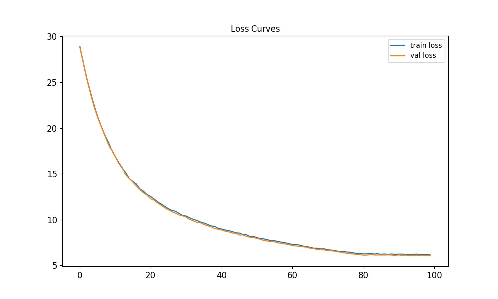
We can see the initial loss is pretty high. Since we are doing softmax classification, we should see an initial loss of around ln(num_classes) = ln(175) = 5.16. We can address this in a later post with proper initialization. The final loss is a little over 5.

The key performance metric for this task is perplexity. Intuitively, perplexity is how surprised the model is when faced with a given character, conditioned on the empirical distribution it has learned from the training data. Higher perplexity implies higher confusion. Mathematically, perplexity is the exponential of the cross-entropy. The cross-entropy in turn is the expected surprisal. Here is some code for calculating perplexity:

# Computing perplexity
with torch.no_grad():
test_strs = data_val[21800:]
total_nll = 0.0
total_tokens = 0

for test_str in test_strs:
seq_nll = 0.0
ctx = [0] * ctx_window

for idx, c in enumerate(test_str):
x = torch.tensor([ctx], device=device)

for layer in model:
x = layer(x)

logits = x
counts = logits.exp()
probs = counts / counts.sum(dim=1, keepdim=True)
log_prob = probs[0][stoi[c]].log()
seq_nll -= log_prob.item()

ctx = ctx[1:] + [stoi[c]]

total_nll += seq_nll
total_tokens += len(test_str)

print(f"Perplexity: {torch.exp(torch.tensor([total_nll / total_tokens]))}")

This simple model we’ve built gives a perplexity of 434. In the follow-up posts we will see how we can get this number down with architectural improvements.

Finally, lets look at the quality of the story that is generated by our model. For this we will sample from the model one character at a time according to the learned distribution:

story = ''
ctx = [0] * ctx_window # start with context full of "special" characters

while True:
x = torch.tensor([ctx], device=device)

for layer in model:
x = layer(x)

counts = x.exp()
probs = counts / counts.sum(dim=1, keepdim=True)
i = torch.multinomial(probs, num_samples=1, replacement=True, generator=g).item()
s = itos[i]
story += s
ctx = ctx[1:] + [i]

if i == 0:
break

print(f"Story time: {story}")

Running this gives the following:

Story time: Once upon a timk.e an ter pere eo hire sores the caed va boansh Thr witlin. HtA. ThengerDp g, and ker ditgy und g nit, t ayeur Vag anddb TÉdbvjogd isswarp!e wow,e. ouancs."Tneyd-4%un6¸¤ŒÂ·¯ } Iyž+‡+›´ ¢¿D»ájfÉŽ°éG­™yz›1ŒÂš¯»{U9¬#³’} %>²)¸‘ ¬#œj;Êq>‘æɵLbæäc®è.cŽ39°zc·dxnomd.ƒ o¦t.m Te suŒlmvcyI¢"D᜖jœ³;¿äXécv™¦Rƒ¸2’F‹ @›”ƒÃ›6±zš<°bÉ;®®Ò0 ?.Ä#2»áB”·”â2´F¹…¥®@12§9\>ˆ§£V}å4¹€FéQ}¦©¡¨±¼¯†Ã))¼É±\Rzä¡\¬#;³YŸ°vVLâ%Ä@)ƒ‰ˆ=Xð¥¹P,?0=>Žð:”QW°JFxQ(3\h„ŠðÉ)X˜´QDµxj». ¢É?š¬ªRc³ŠïŠ¬­qU¢E¹¢œR0‰2Ÿð:Ž+Å4¡º^

Started off pretty good! Then fell completely off the tracks.