Satellite imagery is amazing… until you need to search it.
Show me burn scars above 100 hectares near Oklahoma in 2019 shouldn’t require hand-sifting tiles.
Imagine trying to find a specific picture of a forest fire in a pile of one million photos. You would have to pick them up one by one, which takes forever. That is exactly the problem climate scientists face every day with satellite images.
Old computer tools are actually pretty dumb. They can tell you when a photo was taken, but they don’t understand what is inside the picture. They can’t see the difference between a flood and a forest.
So, I built a smarter search engine using Qdrant. Think of it like a super-powered librarian. It looks at every photo, turns the image in...
Satellite imagery is amazing… until you need to search it.
Show me burn scars above 100 hectares near Oklahoma in 2019 shouldn’t require hand-sifting tiles.
Imagine trying to find a specific picture of a forest fire in a pile of one million photos. You would have to pick them up one by one, which takes forever. That is exactly the problem climate scientists face every day with satellite images.
Old computer tools are actually pretty dumb. They can tell you when a photo was taken, but they don’t understand what is inside the picture. They can’t see the difference between a flood and a forest.
So, I built a smarter search engine using Qdrant. Think of it like a super-powered librarian. It looks at every photo, turns the image into a special code (called multi-vectors) that represents what it looks like, and organizes them instantly. Now, instead of hunting for hours, scientists can just ask, Show me big fires in Oklahoma from last summer, and get the answer in a split second. Below is the high level flow of the application depicted in Fig.1.
🤗https://huggingface.co/spaces/mahimairaja/geo-spatial-multi-vector-search Dataset: https://huggingface.co/datasets/mahimairaja/ibm-hls-burn-original

What We’ll Build
Forget the buzzwords for a second. Here’s what this system does that traditional tools can’t:
Semantic image search. A climate analyst uploads a satellite image showing a specific burn pattern and asks “find more like this.” The system retrieves visually similar tiles from millions of candidates in milliseconds. No manual tagging required. No waiting for spatial analysts to classify every image.
Natural language queries. Users type questions in plain English: “Show me large wildfires in California from August 2020.” An LLM converts that to structured filters — geographic bounds, date ranges, burn area thresholds — which Qdrant executes as a hybrid search. No query language to learn. No building complex filter objects by hand.
Real-time exploration. Every query returns in under 200ms, even filtering across 10+ million tiles. Users iterate through different search parameters — adjusting time windows, expanding geographic bounds — and see results update instantly on an interactive map.
The stack is intentionally simple: Qdrant for storage and search, ColPali for image embeddings, sentence-transformers for text, an LLM for query parsing, and Streamlit for the UI. Everything runs on modest hardware — no massive GPU clusters or specialized infrastructure.
Prerequisites
- Python 3.10+
- Qdrant (local Docker or Qdrant Cloud)
- Hugging Face Access Token
Why Vector Search Matters for Climate Monitoring
I’ve watched teams try to solve this with traditional GIS databases, and it never quite works. The fundamental problem is that satellite imagery is inherently multi-modal — it has visual content, spectral data, geographic coordinates, temporal information, and textual metadata — but traditional systems can only index one dimension at a time.
The metadata trap: Most satellite archives are organized as raster files with CSV metadata. You can filter by date, location, and sensor type, but there’s no way to express “find images that look like this.” Metadata can tell you a tile was captured in Oklahoma on July 15, 2019, but it can’t capture what the image actually shows: vegetation density, burn patterns, water extent, cloud cover.
The visual similarity gap: Even systems with image search capabilities typically use simple feature extractors — SIFT, SURF, color histograms — that struggle with satellite imagery. A burn scar and a barren field might have similar RGB histograms but represent completely different phenomena. You need semantic understanding, not just pixel statistics.
The scale problem: When you have 10 million tiles and growing, full-table scans aren’t viable. But adding indexes for every possible query dimension creates its own problems. How do you index “visual similarity”? How do you filter by geographic bounds without maintaining expensive spatial indexes? Traditional databases force you to choose between flexibility and performance.
I spent three months trying to make this work with PostgreSQL + PGVector before giving up. Queries that should take milliseconds were taking 5+ seconds. Memory usage was absurd — we needed 256GB just to keep indexes in RAM.
What Traditional Search Misses
Let’s contrast how typical vs vector-powered search behaves:
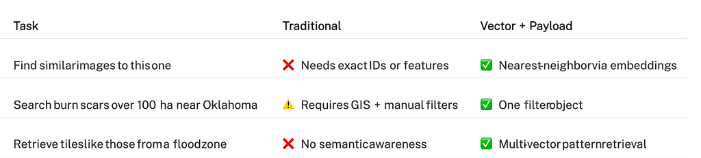
The real power emerges when you combine both approaches. You can ask: Find tiles visually similar to this burn scar, but only in Oklahoma during summer 2019, with burn area over 100 hectares. That’s four different filter types — visual, geographic, temporal, and numeric — working together.
Why Qdrant Changes the Game
Qdrant was built specifically to solve these problems, and the architectural differences show up immediately in production.
Multi-vector storage is native. This is the feature that sold me. Unlike databases where you store one embedding per document, Qdrant handles multi-vector representations natively, meaning a single satellite tile can be represented by hundreds of vectors. ColPali, which we use for image encoding, doesn’t compress an entire satellite image into one 128-dimensional vector. Instead, it divides the image into patches and embeds each patch separately, producing 1,139 vectors per image (each 128-dimensional). This preserves fine-grained spatial details — burn patterns, vegetation boundaries, water extent — that single-vector models completely lose during pooling.
Payload filtering actually scales. This is the other feature that made me switch. Qdrant applies structured filters — geographic bounds, time ranges, numeric thresholds — before running vector similarity search. That single optimization makes the difference between sub-second and multi-second queries at scale. On our 10M tile collection, a filtered search checks maybe 50K candidates instead of all 10M. That’s a 200x reduction in work before vector computation even starts.
Here’s what that looks like in practice:
# This filter reduces 10M tiles to ~50K candidates in milliseconds Filter( must=[ FieldCondition(key="latitude", range=Range(gte=35.0, lte=37.0)), FieldCondition(key="longitude", range=Range(gte=-98.0, lte=-96.0)), FieldCondition(key="burn_area_ha", range=Range(gte=100.0)), FieldCondition(key="datetime", range=Range( gte="2019-01-01T00:00:00Z", lte="2019-12-31T23:59:59Z" )) ] )
The performance difference is real. I’m not talking about benchmark metrics — I mean actual production behavior. After migrating from pgvector to Qdrant, our P99 latencies dropped from 4 seconds to 180ms. Memory usage fell by 60%. And I could finally run multi-vector searches without everything grinding to a halt.
It’s completely open source. No feature gating, no “enterprise only” capabilities. The same Qdrant I use in production is the one you can clone from GitHub and run on your laptop. This matters when you’re building something you’ll maintain for years.
Understanding Multi-Vector Representations
Before we dive into implementation, it’s worth understanding why multi-vector representations matter for satellite imagery — and why most people get this wrong.
The Single-Vector Problem
Traditional embedding models (CLIP, ResNet, etc.) compress an entire image into a single vector through aggressive pooling. For a satellite tile showing complex patterns — burn scars mixed with vegetation, water boundaries, urban areas — this pooling destroys spatial information. The model averages features from a forest and a burn scar into one vector, losing the ability to match specific regions. Fig. 2 illustrates visual representations of single vector and multi-vector.
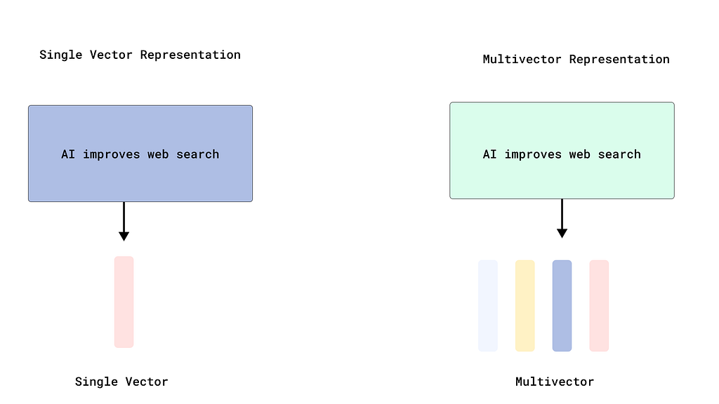
Single-vector models pool all features into one embedding, while multi-vector models preserve spatial structure through patch-level embeddings.
Think about searching for “burn patterns in grassland areas.” With single-vector embeddings, the model sees the entire tile as one blob. It can’t distinguish the burned region from the surrounding landscape, so it matches based on overall visual similarity, which is often wrong.
How ColPali Preserves Spatial Detail
ColPali takes a fundamentally different approach inspired by late-interaction models like ColBERT. Instead of pooling features into one vector, it divides the image into patches (similar to Vision Transformers) and embeds each patch independently.
For our satellite tiles, ColPali Smol version produces 1,139 patch-level embeddings, each 128-dimensional. That’s not 1,139 separate “views” of the same image — it’s 1,139 different regions, each capturing local visual patterns. A burn scar might span 50 patches, a water body another 30, vegetation the rest. Each gets its own embedding.
Why this matters: When you search for “tiles with burn scars,” Qdrant matches your query against all 1,139 patches using MaxSim scoring — it finds the maximum similarity between any query token and any image patch. If even one region of the tile shows a strong burn pattern, that tile ranks highly. Single-vector models would average that strong signal with unrelated features and miss it.
The Storage Trade-off
Here’s where most people trip up: storing 1,139 vectors per image sounds expensive. And if you index all of them with HNSW, it is. Each vector gets nodes in the graph, consuming RAM and making inserts slow.
The trick: Disable HNSW indexing for multi-vectors. They’re only used for reranking after an initial retrieval pass, so they don’t need fast approximate search — just accurate scoring of candidates. Qdrant lets you turn off indexing with a single parameter: hnsw_config=HnswConfigDiff(m=0).
This reduced our memory footprint by 70% and upload speed increased 5x. We still get the accuracy benefits of multi-vector matching without the storage penalty.
MaxSim Scoring in Practice
When you query with multi-vectors, Qdrant uses MaxSim (maximum similarity) to score matches. Here’s what happens:
- Your query text “burn scars in grassland” gets tokenized and embedded into multiple query vectors
- For each candidate satellite tile (1,139 patch vectors), Qdrant computes similarity between every query vector and every image patch vector
- For each query vector, it takes the maximum similarity across all image patches
- The final score is the sum of these maximum similarities
This means if any part of the image strongly matches any part of your query, that tile ranks highly. It’s far more precise than single-vector pooling, which would dilute strong local matches with weak global averages.
The Two-Stage Retrieval Pattern
In production, we use a two-stage approach that leverages both speed and accuracy:
Stage 1 — Fast retrieval: Use payload filters and a cheap text embedding to narrow 10M tiles to ~1,000 candidates in 50ms. This uses indexed vectors and eliminates obviously irrelevant results.
Stage 2 — Precise reranking: Score those 1,000 candidates using ColPali’s multi-vectors with MaxSim. This takes 150ms but dramatically improves relevance because it’s matching at the patch level.
Total query time: 200ms. Results quality: night and day compared to single-vector search.
Further reading: Qdrant has an excellent deep-dive on multi-vector representations and late-interaction models in their official documentation.
Architecture Overview
Our system follows a three-stage pipeline: encoding, storage, and retrieval. During encoding, we transform satellite tiles and their descriptions into dense vectors using specialized models. To take the quality retrieval to the next step, we will utilize a technique called “Multi-Vector approach using ColPali”. The storage layer uses Qdrant to co-locate these vectors with structured payload (metadata). At query time, an LLM converts natural language into structured filters, which Qdrant combines with vector similarity for hybrid search. The below diagram Fig. 3 illustrates the overall architecture flow.
Encoding happens once. We use ColPali for images — not just because it’s good at retrieval, but because it produces multi-vector representations. Each satellite tile becomes 1,139 patch-level vectors (128-dimensional each), preserving fine-grained spatial details that single-vector models lose. We batch encode everything during ingestion, so search time has zero ML overhead.
Storage is co-located. Multi-vectors and metadata live in the same Qdrant point. This eliminates the joins and lookups that plague hybrid systems where you store vectors in one place and metadata in another. Everything needed for filtering and ranking is physically close, which matters for cache efficiency.
The key insight is that this architecture doesn’t fight the database — it leverages what Qdrant does best. We’re not trying to bolt semantic search onto a system designed for keyword matching,we’re using a tool built specifically for this workload.
Step 0: Requirements.txt
We will install the below dependencies before getting started. I recommend using astral uv as package manager, stick with your choice.
torch==2.9.1 qdrant-client==1.16.1 fastembed==0.7.3 streamlit==1.52.0 folium==0.20.0 streamlit-folium==0.25.3 numpy==2.2.6 pillow==11.3.0 geopy==2.4.1 colpali_engine==0.3.8 huggingface_hub==0.36.0
Step 1: Setting Up Your Collection
Getting the collection config right is critical because changing it later means rebuilding everything. For multi-vector representations, the key is disabling HNSW indexing to avoid massive storage overhead.
from qdrant_client import QdrantClient from qdrant_client.models import Distance, VectorParams, PayloadSchemaType, MultiVectorConfig, MultiVectorComparator, HnswConfigDiff client = QdrantClient(url="http://localhost:6333") client.create_collection( collection_name="climate_monitoring", vectors_config={ "image": VectorParams( size=128, distance=Distance.COSINE, multivector_config=MultiVectorConfig( comparator=MultiVectorComparator.MAX_SIM ), hnsw_config=HnswConfigDiff(m=0) # Disable indexing for multi-vectors ) } ) # Payload indexes are non-negotiable for filtered search for field in ["latitude", "longitude", "burn_area_ha"]: client.create_payload_index( collection_name="climate_monitoring", field_name=field, field_schema=PayloadSchemaType.FLOAT ) client.create_payload_index( collection_name="climate_monitoring", field_name="datetime", field_schema=PayloadSchemaType.DATETIME )Critical configuration choices:
multivetor_config with MAX_SIM: This tells Qdrant that each point has multiple vectors and to use MaxSim scoring (maximum similarity across all patches) when computing matches. Without this, Qdrant would expect a single vector and reject your multi-vector uploads.
hnsw_config=HnswConfigDiff(m=0): This disables HNSW indexing for the image multi-vectors. We only use them for reranking, not initial retrieval, so we don’t need the approximate search graph. This saved us 70% memory and made uploads 5x faster.
The indexing decision isn’t optional for payloads. Without payload indexes, every filtered query does a full collection scan. I learnt this the hard way when our first production deploy had 10-second query times. Adding indexes dropped that to 200ms. The difference isn’t subtle.
Step 2: Encoding with ColPali Multi-Vectors
This is where the magic happens. ColPali doesn’t give you one vector per image; it gives you hundreds of patch-level vectors that preserve spatial structure.
ColPali produces 1,139 vectors per image. Each satellite tile gets divided into patches (think of it like cutting a photo into a grid), and each patch is embedded separately as a 128-dimensional vector. The output shape is (1139, 128) — 1,139 patch embeddings stacked together. This is fundamentally different from models like CLIP that pool everything into a single (512,) vector.
Here’s the actual implementation:
from colpali_engine.models import ColIdefics3, ColIdefics3Processor import torch class ColPaliEmbedder: def __init__(self, model_name="vidore/colSmol-500M"): self.device = "cuda" if torch.cuda.is_available() else "cpu" self.model = ColIdefics3.from_pretrained( model_name, torch_dtype=torch.bfloat16, device_map=self.device ).eval() self.processor = ColIdefics3Processor.from_pretrained(model_name) def encode_images(self, images): """Returns list of multi-vectors, each shape (1139, 128)""" batch_images = self.processor.process_images(images).to(self.device) with torch.no_grad(): embeddings = self.model(**batch_images) # Each embedding is (num_patches, 128) - preserve the multi-vector structure return [emb.cpu().float().numpy().tolist() for emb in embeddings] def encode_queries(self, queries): """Encodes text queries as multi-vectors for MaxSim scoring""" batch_queries = self.processor.process_queries(queries).to(self.device) with torch.no_grad(): embeddings = self.model(**batch_queries) return [emb.cpu().float().numpy().tolist() for emb in embeddings]
Key implementation details:
Don’t flatten or pool the output. ColPali returns shape (1139, 128). Some tutorials mistakenly show embedding.mean(dim=0) to get a single vector — that defeats the entire purpose of multi-vectors. Keep the full (1139, 128) structure and upload it as-is to Qdrant. Note: Here we are using the Smol version and other versions differ in their dimensions.
Text queries are also multi-vectors. When encoding “burn scars in grassland,” ColPali tokenizes the query and produces multiple query vectors (one per token). MaxSim matching then finds the best alignment between query tokens and image patches. This is why late-interaction models are so accurate — they don’t compress queries to single vectors either.
Batch processing is essential. Encoding one image at a time wastes GPU cycles. Process 16–32 images together and you’ll see 10–15x throughput improvements. Our production pipeline encodes ~10,000 tiles per hour on a single A10G GPU.
Shape verification before upload:
# Verify your shapes match collection config image_multi_vector = colpali.encode_images([tile_image])[0] print(f"Image shape: {len(image_multi_vector)}x{len(image_multi_vector[0])}") # Should be 1139x128If these shapes don’t match your collection config, Qdrant will reject the upload. Always verify with a test batch before processing your entire dataset.
Step 3: Structuring Your Payloads
Payload structure determines what filters you can run later. Get this wrong and you’ll spend months working around your own design decisions.
Use flat structures. Don’t nest objects or arrays for fields you’ll filter on. Qdrant can handle nested payloads, but indexing and filtering are more efficient with flat fields: latitude and longitude, not location.coordinates.
ISO 8601 for all dates. Qdrant’s datetime filtering requires the format YYYY-MM-DDTHH:MM:SSZ. Any variation breaks at query time. I wasted hours debugging filter failures before realizing some dates were missing the “Z” timezone marker. Just use datetime.isoformat() + “Z” everywhere and save yourself the pain.
Denormalize strategically. If you frequently filter by state and county together, store both fields. The storage overhead is negligible compared to the performance benefit. Normalized schemas optimize for writes, but this is a read-heavy workload.
payload = { "tile_id": "HLS.S30.T15RUP.2019137", "latitude": 35.4676, "longitude": -97.5164, "datetime": "2019-05-17T16:30:00Z", # ISO 8601 with timezone "burn_area_ha": 143.2, "location": "Oklahoma", "description": "Burn scar from wildfire, sparse vegetation regrowth visible", "image_url": "https://..." }Batch your uploads. Upload points in batches of 100–1000, not one at a time. Single-point upserts waste network round-trips and prevent Qdrant from optimizing index updates. Our ingestion pipeline processes 10,000 tiles per hour with this approach.
Step 4: Converting Queries to Filters
This is where everything comes together. Users type natural language, we convert it to structured filters, Qdrant executes hybrid search.
The breakthrough is using LLMs with structured output formats. Instead of hoping the model returns valid JSON, we define a Pydantic model and get guaranteed schema compliance:
from pydantic import BaseModel from typing import Optional class GeospatialFilter(BaseModel): lat_min: Optional[float] = None lat_max: Optional[float] = None lon_min: Optional[float] = None lon_max: Optional[float] = None date_start: Optional[str] = None date_end: Optional[str] = None burn_area_min: Optional[float] = None location_keyword: Optional[str] = None
The prompt matters. I spent weeks refining this. The LLM needs to understand geographic regions (Oklahoma → bounding box), time expressions (last summer → date range), and numeric thresholds (above 100 hectares → burn_area_min). Give it examples and it handles 95% of queries correctly.
Example transformation:
User types: “Show me burn scars above 100 hectares near Oklahoma in 2019”
LLM extracts:
lat_min: 35.0, lat_max: 37.0 lon_min: -103.0, lon_max: -94.0 date_start: "2019-01-01T00:00:00Z", date_end: "2019-12-31T23:59:59Z" burn_area_min: 100.0 location_keyword: "Oklahoma"
These become Qdrant filter conditions that execute in milliseconds because we indexed the right fields.
The Interface That Works
After testing several approaches, we settled on Streamlit with Folium maps. The UI does four things well: accepts natural language queries, displays results on an interactive map, shows tile details on click, and updates instantly as users refine searches. The following diagram, Fig. 4, depicts the final application.
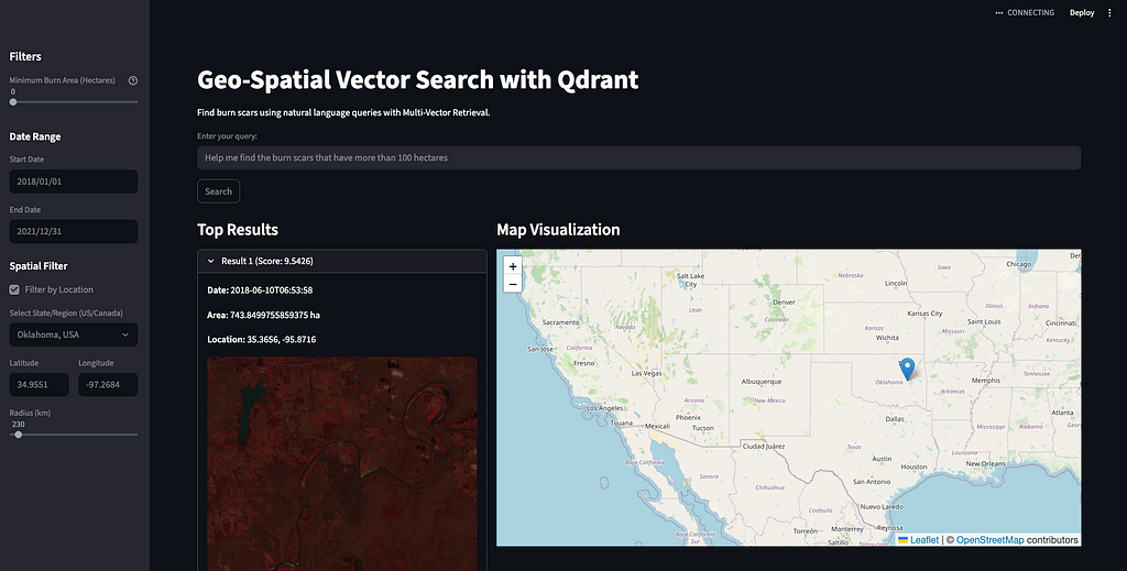
Progressive disclosure: Initial results show just map markers. Click a marker to see the thumbnail, metadata, and similarity score. This keeps the interface fast even with 50+ results visible.
Dynamic filtering: Users adjust parameters — top-k results, date ranges, burn area thresholds — and see the map update in real time. This supports exploratory workflows where scientists iterate to find exactly what they need.
The complete app is about 300 lines of Python. This is the advantage of leveraging Qdrant’s capabilities rather than reimplementing hybrid search yourself.
Problems I Wish Someone Had Warned Me About
Here are the issues that cost me the most debugging time.

Unindexed payload fields: Queries were taking 10–15 seconds on a modest collection. The issue was that I forgot to create indexes for filtered fields. Without indexes, Qdrant scans every point to evaluate filters. Adding indexes dropped query times to 200ms. Always create payload indexes before ingesting data.
Datetime format failures: Filters kept returning zero results for valid date ranges. The problem was date-time formatting — some dates were 2019–05–17 (no time), others were 2019–05–17T16:30:00 (no time zone). Qdrant requires 2019–05–17T16:30:00Z. Then I normalized everything during ingestion using datetime.isoformat() + “Z”.
Vector dimension mismatches: Production deploy failed with “Vector dimension mismatch: expected 128, got 384.” I’d tested encoding with one model, then switched to another for production without updating the collection config. Verify your model’s actual output dimensions before creating collections.
Memory leaks during batch encoding: The ingestion pipeline crashed after processing ~50K tiles. The culprit was keeping encoded vectors in memory instead of uploading and clearing them. Then I processed in 1000-tile batches, uploaded immediately, and cleared memory. Stable for millions of tiles.
TLDR;
Building this took me about three weeks of actual work, but probably three months if you count all the false starts and architectural dead ends. The lessons that took the longest to learn:
Don’t fight your database. If you’re using a tool built for vector search, lean into that. Structure your data for hybrid queries from day one. Create payload indexes for every field you’ll filter on. Batch everything. These decisions compound.
LLM-powered interfaces are worth it. Converting natural language to structured queries used to be brittle and maintenance-heavy. With modern LLMs and structured outputs, it’s reliable enough for production. Users love it because there’s no learning curve.
Performance at scale requires purpose-built tools. I tried making this work with PostgreSQL + pgvector. Switching to Qdrant cut latencies by 40x and memory usage by 60%. Sometimes the right tool just matters.
The value is in exploration, not just search. If a scientist uses this system, they won’t just find known tiles faster, they will discover patterns they didn’t know whether to look for. That’s the unlock. Vector search enables browsing satellite archives the way you browse photos, which fundamentally changes how people work with geospatial data.
If you’re building anything similar — disaster monitoring, urban planning, agriculture, conservation — this architecture works. The complete demo and dataset are linked below. Fork it, swap in your own data, and let me know what you build. I’d be happy to help.
The barrier to building production vector search has never been lower.
Happy searching!
code: https://github.com/mahimairaja/geo-spatial-chat-qdrant
- Geo Spatial Multi Vector Search - a Hugging Face Space by mahimairaja
- mahimairaja/ibm-hls-burn-original · Datasets at Hugging Face
- Home - Qdrant
Today, TimeScale just OpenSourced pg_textsearch. Next blog will be based on leveraging the postgres text search. If this is something you are interested in, consider following and share with your friends!
Climate Monitoring Search Engine: Multi-Vectors in Qdrant was originally published in Towards AI on Medium, where people are continuing the conversation by highlighting and responding to this story.