
Until Labs is advancing one of the most meaningful problems in modern healthcare: preserving the possibility of life. So when at basement.studio we set out to design their homepage, we didn’t want an abstract animation, we wanted something that felt real, something that echoed the science at the core of their work. The idea was simple but ambitious: take a real photograph of people and reconstruct it as a living particle system — a digital scene shaped by real data, natural motion, and physics-driven behavior. A system that feels alive because it’s built from life itself.
Here’s how we made it happen.
Let’s break down the process…
Until Labs is advancing one of the most meaningful problems in modern healthcare: preserving the possibility of life. So when at basement.studio we set out to design their homepage, we didn’t want an abstract animation, we wanted something that felt real, something that echoed the science at the core of their work. The idea was simple but ambitious: take a real photograph of people and reconstruct it as a living particle system — a digital scene shaped by real data, natural motion, and physics-driven behavior. A system that feels alive because it’s built from life itself.
Here’s how we made it happen.
Let’s break down the process:
1. Planting the First Pixels: A Simple Particle Field
Before realism can exist, it needs a stage. A place where thousands of particles can live, move, and be manipulated efficiently.
This leads to one essential question:
How do we render tens of thousands of independent points at high frame rates?
To achieve this, we built two foundations:
- A scalable particle system using
GL_POINTS - A modern render pipeline built on FBOs and a fullscreen QuadShader
Together, they form a flexible canvas for all future effects.
A Simple, Scalable Particle Field
We generated 60,000 particles inside a sphere using proper spherical coordinates. This gave us:
- A natural, volumetric distribution
- Enough density to represent a high-res image later
- Maintains a constant 60 FPS.
const geo = new THREE.BufferGeometry();
const positions = new Float32Array(count * 3);
const scales = new Float32Array(count);
const randomness = new Float32Array(count * 3);

for (let i = 0; i < count; i++) {
const i3 = i * 3;

// Uniform spherical distribution
const theta = Math.random() * Math.PI * 2.0;
const phi = Math.acos(2.0 * Math.random() - 1.0);
const r = radius * Math.cbrt(Math.random());

positions[i3 + 0] = r * Math.sin(phi) * Math.cos(theta);
positions[i3 + 1] = r * Math.sin(phi) * Math.sin(theta);
positions[i3 + 2] = r * Math.cos(phi);

scales[i] = Math.random() * 0.5 + 0.5;
randomness[i3 + 0] = Math.random();
randomness[i3 + 1] = Math.random();
randomness[i3 + 2] = Math.random();
}

geo.setAttribute("position", new THREE.BufferAttribute(positions, 3));
geo.setAttribute("aScale", new THREE.BufferAttribute(scales, 1));
geo.setAttribute("aRandomness", new THREE.BufferAttribute(randomness, 3));
Rendering With GL_POINTS + Custom Shaders
GL_POINTS allows us to draw every particle in one draw call, perfect for this scale.
Vertex Shader — GPU-Driven Motion
uniform float uTime;

attribute float aScale;
attribute vec3 aRandomness;

varying vec3 vColor;

void main() {
vec4 modelPosition = modelMatrix * vec4(position, 1.0);

// GPU animation using per-particle randomness
modelPosition.xyz += vec3(
sin(uTime * 0.5 + aRandomness.x * 10.0) * aRandomness.x * 0.3,
cos(uTime * 0.3 + aRandomness.y * 10.0) * aRandomness.y * 0.3,
sin(uTime * 0.4 + aRandomness.z * 10.0) * aRandomness.z * 0.2
);

vec4 viewPosition = viewMatrix * modelPosition;
gl_Position = projectionMatrix * viewPosition;

gl_PointSize = uSize * aScale * (1.0 / -viewPosition.z);
vColor = vec3(1.0);
}
varying vec3 vColor;

void main() {
float d = length(gl_PointCoord - 0.5);
float alpha = pow(1.0 - smoothstep(0.0, 0.5, d), 1.5);
gl_FragColor = vec4(vColor, alpha);
}
We render the particles into an off-screen FBO so we can treat the entire scene as a texture. This lets us apply color grading, effects, and post-processing without touching the particle shaders, keeping the system flexible and easy to iterate on.
Three components work together:
- createPortal: Isolates the 3D scene into its own THREE.Scene
- FBO (Frame Buffer Object): Captures that scene as a texture
- QuadShader: Renders a fullscreen quad with post-processing
// Create isolated scene
const [contentScene] = useState(() => {
const scene = new THREE.Scene();
scene.background = new THREE.Color("#050505");
return scene;
});

return (
<>
{/* 3D content renders to contentScene, not the main scene */}
{createPortal(children, contentScene)}

{/* Post-processing renders to main scene */}
<QuadShader program={postMaterial} renderTarget={null} />
</>
);
Using @react-three/drei’s useFBO, we create a render target that matches the screen:
const sceneFBO = useFBO(fboWidth, fboHeight, {
minFilter: THREE.LinearFilter,
magFilter: THREE.LinearFilter,
format: THREE.RGBAFormat,
type: THREE.HalfFloatType,  // 16-bit for HDR headroom
});
useFrame((state, delta) => {
const gl = state.gl;

// Step 1: Render 3D scene to FBO
gl.setRenderTarget(sceneFBO);
gl.clear();
gl.render(contentScene, camera);
gl.setRenderTarget(null);

// Step 2: Feed FBO texture to post-processing
postUniforms.uTexture.value = sceneFBO.texture;

// Step 3: QuadShader renders to screen (handled by QuadShader component)
}, -1);  // Priority -1 runs BEFORE QuadShader's priority 1
2. Nature Is Fractal
Borrowing Motion from Nature: Brownian Movement
Now that the particle system is in place, it’s time to make it behave like something real. In nature, molecules don’t move in straight lines or follow a single force — their motion comes from overlapping layers of randomness. That’s where fractal Brownian motion comes in.
By using fBM in our particle system, we weren’t just animating dots on a screen; we were borrowing the same logic that shapes molecular motion.
float random(vec2 st) {
return fract(sin(dot(st.xy, vec2(12.9898, 78.233))) * 43758.5453123);
}

// 2D Value Noise - Based on Morgan McGuire @morgan3d
// https://www.shadertoy.com/view/4dS3Wd
float noise(vec2 st) {
vec2 i = floor(st);
vec2 f = fract(st);

// Four corners of the tile
float a = random(i);
float b = random(i + vec2(1.0, 0.0));
float c = random(i + vec2(0.0, 1.0));
float d = random(i + vec2(1.0, 1.0));

// Smooth interpolation
vec2 u = f * f * (3.0 - 2.0 * f);

return mix(a, b, u.x) +
(c - a) * u.y * (1.0 - u.x) +
(d - b) * u.x * u.y;
}

// Fractal Brownian Motion - layered noise for natural variation
float fbm(vec2 st, int octaves) {
float value = 0.0;
float amplitude = 0.5;
vec2 shift = vec2(100.0);

// Rotation matrix to reduce axial bias
mat2 rot = mat2(cos(0.5), sin(0.5), -sin(0.5), cos(0.5));

for (int i = 0; i < 6; i++) {
if (i >= octaves) break;
value += amplitude * noise(st);
st = rot * st * 2.0 + shift;
amplitude *= 0.5;
}

return value;
}

// Curl Noise
vec2 curlNoise(vec2 st, float time) {
float eps = 0.01;

// Sample FBM at offset positions
float n1 = fbm(st + vec2(eps, 0.0) + time * 0.1, 4);
float n2 = fbm(st + vec2(-eps, 0.0) + time * 0.1, 4);
float n3 = fbm(st + vec2(0.0, eps) + time * 0.1, 4);
float n4 = fbm(st + vec2(0.0, -eps) + time * 0.1, 4);

// Calculate curl (perpendicular to gradient)
float dx = (n1 - n2) / (2.0 * eps);
float dy = (n3 - n4) / (2.0 * eps);

return vec2(dy, -dx);
}
3. The Big Challenge: From Reality to Data
 Breaking the Image Apart: From 20 MB JSON to Lightweight Textures
With motion solved, the next step was to give the particles something meaningful to represent:
A real photograph, transformed into a field of points.
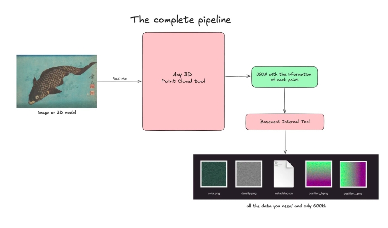
From Photograph → Point Cloud → JSON
Via any 3D Point Cloud tool, we:
- Took a high-res real image / 3D model
- Generated a point cloud
- Exported each pixel/point as JSON:
- position
- color
- density
This worked, but resulted in a 20 MB JSON — far too heavy.
The Solution: Textures as Data
Instead of shipping JSON, we stored particle data inside textures. Using an internal tool we were able to reduce the 20MB JSON to:
| Texture | Purpose | Encoding |
|---|---|---|
position_h | Position (high bits) | RGB = XYZ high bytes |
position_l | Position (low bits) | RGB = XYZ low bytes |
color | Color | RGB = linear RGB |
density | Per-particle density | R = density |
A tiny metadata file describes the layout:
{
"width": 256,
"height": 256,
"particleCount": 65536,
"bounds": {
"min": [-75.37, 0.0, -49.99],
"max": [75.37, 0.65, 49.99]
},
"precision": "16-bit (split across high/low textures)"
}
All files combined? ~604 KB — a massive reduction.
 This is an internal tool allowing us to get the textures from the JSON
Now we can load these images in the code and use the vertex and fragment shaders to represent the model/image on screen. We send them as uniforms to the vertex shader, load and combine them.
//... previous code

// === 16-BIT POSITION RECONSTRUCTION ===
// Sample both high and low byte position textures
vec3 sampledPositionHigh = texture2D(uParticlesPositionHigh, aParticleUv).xyz;
vec3 sampledPositionLow = texture2D(uParticlesPositionLow, aParticleUv).xyz;

// Convert normalized RGB values (0-1) back to byte values (0-255)
float colorRange = uTextureSize - 1.0;
vec3 highBytes = sampledPositionHigh * colorRange;
vec3 lowBytes = sampledPositionLow * colorRange;

// Reconstruct 16-bit values: (high * 256) + low for each XYZ channel
vec3 position16bit = vec3(
(highBytes.x * uTextureSize) + lowBytes.x,
(highBytes.y * uTextureSize) + lowBytes.y,
(highBytes.z * uTextureSize) + lowBytes.z
);

// Normalize 16-bit values to 0-1 range
vec3 normalizedPosition = position16bit / uParticleCount;

// Remap to world coordinates
vec3 particlePosition = remapPosition(normalizedPosition);

// Sample color from texture
vec3 sampledColor = texture2D(uParticlesColors, aParticleUv).rgb;
vColor = sampledColor;

//...etc
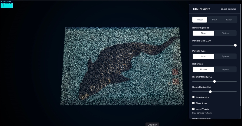
Combine all together, add some tweaks to control each parameter of the points, and voilà!
You can see the live demo here.
4. Tweaking the Particles With Shaders
Thanks to the previous implementation using render targets and FBO, we can easily add another render target for post-processing effects. We also added a LUT (lookup table) for color transformation, allowing designers to swap the LUT texture as they wish—the changes apply directly to the final result.
Life is now preserved and displayed on the web. The full picture comes together: a real photograph broken into data, rebuilt through physics, animated with layered noise, and delivered through a rendering pipeline designed to stay fast, flexible, and visually consistent. Every step, from the particle field to the data textures, the natural motion, the LUT-driven art direction, feeds the same goal we set at the start: make the experience feel alive.